











![Mechanics Livestream 🚂 [Bicen Maths Live 📹] Weds 23rd April, 5pm](https://i.ytimg.com/vi/o4QAlrXk_AY/maxresdefault.jpg)









Polymer chain conformation refers to the spatial arrangement of polymer chains in three-dimensional space, which can be quantified through structural characteristics including contour length (fully extended chain length), root mean square end-to-end distance (scaling as n^0.5 for ideal chains), persistence length (measuring chain stiffness), radius of gyration (average distance from center of mass), and hydrodynamic radius (diffusion-related size). These single-chain properties directly influence bulk material properties such as solution behavior, melt characteristics, swelling, crystallinity, and viscoelasticity, making them fundamental to understanding polymer structure-property relationships.
Chain Conformation & Structural Characteristics in Polymers
Added:Basic Polymer Chemistry: Understanding of polymer chains, monomers, repeating units, and molecular weight distribution.
Statistical Mechanics and Probability: Concepts of random walks, statistical averages, and probability distribution functions.
Stereochemistry and Molecular Geometry: Familiarity with bond lengths, bond angles, dihedral angles, and steric hindrance in polymer backbones.
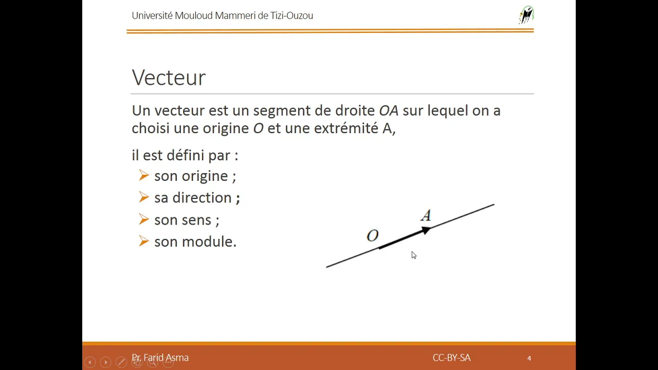
Vector Calculus and Mechanics: Proficiency with vector operations (like dot products) and the concept of center of mass (crucial for understanding radius of gyration).
Thermodynamics of Polymer Solutions: Exploring Flory-Huggins theory, polymer-solvent interactions, and the concept of theta solvents.
Entropic Elasticity and Rubber Elasticity: Understanding how conformational entropy changes relate to the macroscopic elasticity of elastomers.
Experimental Characterization Methods: Learning how to experimentally measure chain size and conformation using techniques like Light Scattering (SLS), SAXS, and SANS.
Polymer Dynamics and Rheology: Studying the motion of polymer chains in solutions and melts through the Rouse, Zimm, and reptation models.
231 views1likes1:10:03Original Release: 2026-04-10
Hello, welcome back to the course on polymeric biomeaterials. We are uh still looking at structure property relationships and in today's lecture we will be focusing on chain confirmation and structural characteristics.
Now in the last lecture we were broadly looking at molar mass and we were trying to connect it to the degree of polymerization or the average number of mers in the chain and we looked at some average properties for a number of chains. We looked at distributions there. The question we were asking was what is the size of these chains?
Now in this lecture we will ask that same question but from a slightly different perspective. In the previous lecture we were interested in just the chain length distribution of chain lengths the relative contributions of the different weight fractions to the overall molar mass and so on. In this lecture, we're going to ask how do these chains orient themselves in threedimensional space for which we'll have to look at something called chain confirmations.
So here the focus of this lecture will be looking at a single macroolecular chain but then asking how do confirmations result in different sizes in 3D for a polymer. And to understand that the starting point for us will be what you will call an ideal chain with its own set of assumptions uh which is one of the simplest ways to think about these chains and then we can add realistic constraints to a model that can describe the ideal chain and then we can try to see how the sizes can change in 3D and we will also look at a few different structural characteristics uh numbers essentially that can be used to quantify these sizes such as end to- end distance, persistence length, radius of geration and hydrodnamic radius and then ultimately as always we will connect how these single chain properties or characteristics can be connected to bulk properties. Now the philosophy with this lecture is to have a good physical understanding of all these structural characteristics. Our goal is not to derive from scratch each of these u formula etc. What we will do primarily is focus on understanding from a physical perspective from a conceptual perspective the size of a macroolelecule from a single chain perspective. Later I will also provide a reference in case you're interested in looking at detailed derivations for some of these things.
So we will start with that that question first which is how big is a macroolelecule or a polymer really in 3D. Now for that we will start with our familiar example of polyethylene of say molar mass 280,000 g per mole. On the left side you have ethylene which is simply 28 g per mole and let's assume n is 10,000.
This will lead to polyethylene of molecular weight 280,000 g per mole.
And can you try and speculate how many carbonarbon bonds will be there in this molecule?
Uh if you guessed it right, this should contain 20,000 carbonarbon bonds in the backbone.
Now if you start with this as an example, we will now consider two extreme length scales here in 3D. One is this chain can be thought of in one extreme as fully stretched out and perfectly linear from end to end.
That would be what we would call the contour length which is this chain fully stretched out from end to end.
The other extreme is the chain is completely collapsed and forms a dense globule where you can now approximate it as a sphere and you can talk about an equivalent sphere radius.
So these would be considered the two extremes for this. Now let's dig a little bit deeper and ask can we come up with some numbers some quantities that can describe both contour length and this sphere radius and try to understand what the differences in these extremities are.
So we'll first begin with looking at the linear or the fully extended chain.
Now there is an easy way for us to approximate the size of this based on the length of the carbonarbon bond. So if you approximate the carbonarbon bond length as being roughly about.15 nanometers which is an approximation and if you consider for the example given uh earlier with 20,000 cc bonds then the contour length from one end of the polymer to the other end in the fully extended uh stretched chain state would be 20,000 time.15 nanometers which will roughly be about 3 microns.
Um and to get a sense of what 3 microns is is um you simply have to consider the fact that a cell uh is about a small cell would be about two times that size.
A red blood cell for example will be about 5 to 6 microns. So this lens scale we're getting this 3 micron lens scale is uh about half that size. So same order of magnitude.
Um while this might seem like an approximation that we're doing, it's a very useful exercise that we will often do uh not just in this course but in engineering in general which is order of magnitude estimates where uh you're not so interested in the details of the calculations but you're interested interested in understanding uh the physical significance of numbers or to get an idea of where you lie on that spectrum. Uh the details are very important uh when you solve problems or when you're designing something. But from a for a conceptual understanding, it is often times the order of magnitude estimate that will really help you get a good sense of uh the physical significance of the numbers you're dealing with. So that's sort of what we're trying to do here. So note down this length scale here for the contour length. The other extreme is for the sphere or the dense globule.
Right? Now if you approximate that uh shape as a sphere. One can think of a length scale associated with it as being equivalent to a sphere radius.
And to get radius you'll have to get uh get that from volume. And for volume uh you'll have to rely upon mass and density. So again we will do that same thing that we did earlier for the fully extended chain which is to do back up the envelope uh calculations to get a sense of the order of magnitude of what we're dealing with here. So if you assume that the bulk density of uh the density of bulk polyethylene is about.9 g per cc which is again an approximation and note that that number will change depending on what type of polyethylene you're dealing with.
uh but you can use that as a starting point for this discussion. Then the volume can simply be calculated based on mass over density and accounting for the avagadro number. So you will roughly end up getting about 516 to 520 nanome cube volume for that same chain as the fully extended chain. And if you calculate the equivalent sphere radius uh for that volume you will end up with 5 nanometers.
Note that for the same chain that we saw here which is the linear fully extended chain that exact same chain in uh in the sphere or the dense globial form is giving you giving you a length scale that's three orders of magnitude smaller than the contour length.
Now to get a sense of what that means is if you consider the equivalent sphere radius 5 nanometers as equal to the size of a let's say let's say a basketball whose diameter will roughly be about 10 in let's say if that's the lens scale you're talking about here for the dense globule you're talking about 10,000 in for the linear fully extended chain which would be approximately the length of a basketball court. So for the same chain in one state you're in the fully extended uh state you're talking about the length scale that's of the order of a basketball court.
In the other case for the same chain when it is in the dense globial state you're talking about uh a length scale that is of the order of say the size of a basketball itself. So these are two very very extreme cases for the same check.
Now what explains these differences? How do we come to terms with these very large uh differences in length scales for the same uh chain itself that can be explained based on confirmations that these chains can take.
Firstly, we note that we're using the word confirmations here and we have earlier seen the word configuration.
Note that this is not the same as confirmation.
Configuration is something that cannot be changed after synthesis. It is fixed during synthesis. And uh the only way to change configuration of a polymer molecule is to break primary bonds and reform them which is not easy at all.
Uh so don't confuse that with confirmations here where it is reasonably relatively easy to change confirmations of uh these kinds of systems based on rotations around carbonarbon single bonds. for example as we saw in the case of polyethylene here.
So throughout the chain every CC bond um especially given the fact that the bond is a single bond it can rotate and take on multiple angles and that rotation leads to differences in how the side groups interact with each other across the carbon atoms.
um as we will look at very shortly. So right away you see that uh we are using words like dihedral angle, bond angle etc. And so some terms need to be defined before we proceed further and we will use this example here to define these terms more clearly. So shown here is a cartoon or a schematic representation of a fourcarbon segment of a polyethylene molecule. Now obviously the polyethne molecule is much longer than this and it's going to proceed in both directions and we're looking only at four of those carbons here to get a good understanding of what dihedral angles or torsional angles are and what bond angles are and these carbon atoms are labeled CIUS 2, CI -1, CI and C I + 1. So those are the four carbon atoms.
Now as you can readily appreciate between four carbon atoms we can define three bonds and uh those bonds have their own bond vectors associated with them namely RA IUS1, RA I and RA + 1. So we have four carbon atoms. We have three bonds that we have defined between them each associated with their own bond vectors. So the carbon atoms and the bond vectors should be clear. Now we have two angles that we're talking about here. One is theta which here we're defining as the angle between two bond vectors.
Now if you look up some textbooks uh you might also have seen that theta sometimes is also defined as the bond angle itself wherein for this kind of a system for a carbonarbon single bond that would roughly be 109 5° but the way we are defining theta is not this here what we're doing is if this bond vector vector where to continue this way but projected that way. Theta is defined as the angle between the bond vector here and the bond vector here. Now you can easily see that the way we are defining theta here which is the angle between two bond vectors will simply be 180 minus the bond angle as classically defined which is 109.5. So if you subtract it you will roughly get about 70.5° or 70° roughly uh for the way we are defining theta here for this system.
So that is an important distinction to keep in mind.
The other angle that we are defining here is the dihedral or the torsional angle.
Dihedral angles are typically defined between two planes. And here we have two planes formed by the bonds RA I bonds represented by the bond vectors R(n) and RA and RA and RA + 1.
So you have two set two planes that intersect and the angle formed between them where uh the carbon carbon can rotate is the dihedral angle as shown here. So as you can clearly see theta uh which is the angle between the bond vectors and the dihedral dihedral or the torsional angles are not the same. In fact for a fixed value of theta you can have the dihedral angle go anywhere from 0 to 360. uh why all the while theta being fixed right and although that's true uh the fact that the dihedral angle can go anywhere from 0 to 360 there are specific angles there that are of interest to us from a steric hindrance perspective which we will look at so shown here um are two different ways in which the CC bond is rotated resulting in um at least two different ways um along the potential energy diagram where you have what we call the trans state and the gsh plus state and depending on uh the angle of rotation the gosh itself can produce two states namely gosh plus and gosh minus and just as an example we are looking at trans and gosh plus here. So first of all we note that both of these are representations of different confirmations for the system here and uh these depend uh both upon the thermal energy available uh to the molecule based on temperature as well as uh the relative steric hindrance uh that the atoms will face when they are either in the trans state or in the gosh state.
The trans state uh is represents a global minimum uh in the potential energy diagram where you have the lowest static hindrance because the hydrogens's along the carbon if you look through the bond the hydrogens's are pointing in opposite directions or in other words these two bonds are what we would call collinear resulting in least static hindrance among all the confirmations possible.
Uh the gosh state um is also a staggered state but is a higher energy state than the trans state because there is some level of steric hindrance uh as compared to the trans state among the atoms attached along the carbons as shown in this diagram here. Now for a polythan molecule it may be hard for you to appreciate exactly what is going on here. So just for understanding this a bit better, we will look at the example of uh another fourcarbon molecule that you're probably familiar with um which is butane and shown here are what are called Newman projections which would give you a much better idea of what we're talking about in terms of potential energy diagrams and relative confirmations.
So again you see here we're looking at the dihedral or the torsional angle on the x-axis and then potential energy on the y-axis.
Um so higher up u the state is uh the less favorable energetically favorable it is. And you notice that the T or the trans state represents the global uh minimum. And uh what you what we are shown here is we're looking through the bonds um along the carbonarbon uh backbone. And uh what you see in the trans state is uh it's a fully staggered state sometimes also called an anti-ate where there is absolutely no um hindrance for you to see the atoms attached to the other carbon when you see from this side. So it is in the fully staggered state where uh there is no overlap of the electron clouds which means that um this state is going to be the lowest energy state among all the states possible. Now compare that with the two gosh states. If I rotate this bond 120° this way or that way, you can see that the CH3 has moved this way or that way. And compared to the trans state, this will have a slightly higher energy state because of slightly higher static hindrance um due to the position of uh the atoms along the carbons. Of course, they are still much better than the states represented by these or these where those will represent eclipsed what you would call eclipse states and uh even here there is a subtle difference in these states it energy is even more higher probably the highest among all of them because there is a direct over uh the CH3s will directly be behind one another. So when you look through one's one methile, the other methile will not be visible because it's right behind it and that leads to the maximum uh static hindrance leading to the highest energy state as opposed to these ones where it is a CH3 hydrogen uh kind of an eclipse. So slightly lower energy compared to uh the CH3 CH3 um eclipse.
But again these states because they're higher energy will not be favored uh easily from a steric hindrance perspective.
Now which state or which confirmation a carbonarbon bond wants to be in will like I said earlier depend upon the thermal energy present. If there is sufficient thermal energy for them to move across states they will move. So we can immediately appreciate that in the melt state these confirmations where the temperature is quite high these confirmations will be enabled or even the transitions and uh if you want to get a sense of the ratio of the states uh for the gosh versus the trans uh that's shown by this formula here and you can readily appreciate uh that this two is simply coming from the fact that you have two god states as compared to one trans state and delta E is simply the energy barrier between the trans and the gosh states. Now this should give you a good sense of a single carbonarbon uh bond rotation uh when you think about what confirmations can be favored, what confirmations are less energetically favored and how those can in turn depend on um temperature. Now you can extend this argument to the entire polythine molecule where each carbonarbon bond has the option to do this. Um and you might pause here and think about um will all possible confirmations be uh favored uh for all the carbonarbon bonds equally.
If your intuition is right, you will immediately see that that won't be true.
Now for a chain with 20,000 bonds uh as we saw at every carbonarbon bond step that uh has the possibility for three different confirmations resulting in 3 to the 20,000 possible confirmations.
Now if you think of this molecule sampling or changing uh as a thought exercise uh changing confirmations every one pose second let's say um you will be shocked at how long it will take for it to sample all the confirmations. It will be much larger than the age of the universe itself.
So that should also tell you why the probability of the fully extended all trans state where um everything is fully stretched out uh or the zigzag state is 1 and 10^ the 10,000 um what you can also now start to think about is because all of these states uh are not energetically the same depending on uh energy barriers across states and depending on which state is energetically more favorable under a given set of conditions based on what is the temperature, what are the solvents, you get different kinds of confirmations that are promoted.
Now one thing to note here is uh which we will look at in more detail later in this lecture is to understand that confirmation and chain flexibility are related.
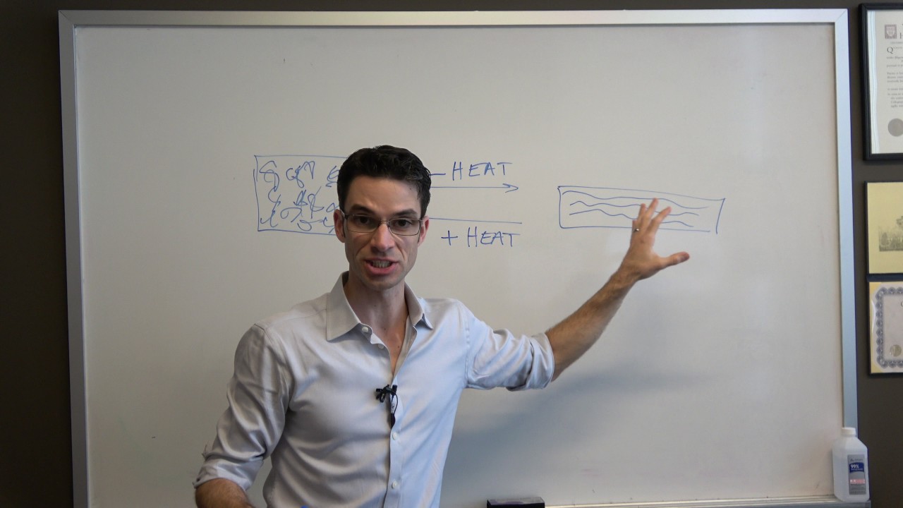
In other words, the all trans uh fully extended state is considered the rod-like state which is considered stiff compared to the introduction of the gosh states which introduces flexibility.
Um that's an important point to keep in mind as we go through uh this lecture because here we are now connecting confirmation to words like flexibility and rod like rigidity. So the association is important here. Also note can you speculate on the presence of say double or triple bonds or the presence of bulky groups along the backbone or if you have high energy barriers what that would do to confirmations?
You can immediately see that these things will restrict the bond rotation and uh will change the way uh the polymer confirmations can happen.
Uh while we are focused here primarily so far on the CC bond, it's important to keep in mind that when you have double bonds or when you have bulky groups in the backbone or on the side, those things can restrict chain rotation.
Now, as you can now clearly start to think about different confirmations, a large number of different sequences of T the trans, G plus the gosh plus, and G minus the gosh minus can cause the chain to wander about in space wherein the typical size that you can think of for this chain or macroolelecule will be intermediate between the fully fully extended chain and the dense sphere.
The fully extended chain uh for example the all trans zigzag state uh is occurs with very low probability as we saw and the dense globule also has a low probability because of multiple confirmations that can be um introduced in each of these bonds. that all trans going from the all trans uh to some flexibility is achieved through the introduction of several gosh uh in between and that is also a function of temperature.
If you have the melt state, if you're working, if you're increasing the temperature, you can now start to think about uh more gosh states being favored.
And uh it's a bit counterintuitive uh because with increase in temperature, you start to think that uh everything increases. So you would think this becomes longer. Actually the opposite happens where with increases in temperature more gosh states are favored. the chain starts to become more flexible and the overall size starts to go down. That's a very interesting aspect in polymers.
So if you now consider just three different temporal snapshots of the same polymer chain, so structurally the same polymer, same chemistry, three different confirmations based on how each carbonarbon bond decides to take up different confirmations.
So what I'm showing here is a temporal snapshot going from left to right. At one time instant it could take up this confirmation. At another time instant it could take up this confirmation. At another time instant it could take up this. So as you can clearly see within energetic constraints you can have billions and billions of confirmations.
So it's very difficult to talk about instantaneous confirmations. Rather we are now interested in averages for which we will have to now think about the polymer as a random coil and this is why if you remember we have talked about the cooked spaghetti analogy for polymers which is a random entangled mass of chains.
A random coil to note is doesn't refer to a specific confirmation but is actually a dynamic and flexible confirmation that represents a statistical distribution of shapes as a function of both temperature and solvent.
So if you think about that same chain now if you zoom out a bit and don't focus so much on the links but look at the chain as a whole. In one instance it could look like this. In another instance it could look like this. In a third instance it could look like this.
These are all uh what we would consider random coils which would again be remember that they would be dynamic and flexible. they're continuously changing because of the solvent and the temperature.
Now we first want to ask how do we understand in terms of sizes uh how do we want to understand uh confirmations of the random coil itself and the overall chain.
Uh for us to look at this in more detail, we have to first define what you will call an ideal chain from which uh or based on which we will develop models uh to understand what we can think of as an average size of this chain.
Now when you hear the word ideal chain you might have you might be familiar very likely with ideal gases where uh ideal gases assume no interactions between uh the molecules.
So these would be molecules for ideal gases. So like ideal gases here there are no interactions between the monomers for an ideal chain. Another very important idea for ideal chains is ideal chains don't assume excluded volume. So extruded volume effects are ignored. Uh we will look at this in more detail uh as we go through u in a later topic what this means. But for now uh one way to understand what extruded volume is is when polymers keep doing this dynamic fluctuation and uh and so on. Um because these molecules occupy volume uh you can't have chains cross path or go through or intersect or no two polymer segments can occupy the same point in space in threedimensional space. So the effective uh size that you get uh for a real chain will be larger than for an ideal chain which does not uh take into account these extruded volume effects.
So in an ideal chain chains can actually cross over right chains can intersect, chains can go on top, they can do all kinds of things which would be considered unphysical.
Is that still okay? As it turns out, it's a great starting point for us to understand how chains behave eventually because we can now start to think about just as we do with ideal gases, we can now start to think about if this is the model for an ideal chain, can we now start imposing constraints based on realistic um considerations and then start to ask what are the deviations from ideal chain behavior. That's one way to think about this. And one of the simplest models we will look at uh for this is called the freely jointed chain model.
um any model uh that you come across the word model itself simply indicates that uh the framework that we're going to come up with is going to reflect some aspect uh physically of the system likely through a mathematical equation and uh all models will have a set of assumptions and uh when those assumptions get violated the model becomes limited. The model becomes no longer applicable. So it's very important when we start looking at models to know what the assumptions or the underlying framework is for the model.
This model like I said is the simplest model for an ideal chain. It cons considers n rigid lengths which would be the bonds between uh the coalent bonds between the mers each with a fixed length of L and L here is a vector.
One very important point to note here is the orientation of one link doesn't affect the next. This is what we would call uncorrelated. What that means is the first link that goes and the next link that comes uh need not have any connection at all in the sense the direction in which the first link points and the direction in which the second link points uh may have no correlation.
Uh does that really happen uh in a polymer? No. But this is the assumption of the ideal chain or the freely jointed chain model.
The other assumption we make here is no restrictions either on the bond angles or on the dihedral angles. Again if you notice here bond angles typically for um carbon carbon uh the tetrahedral angle is typically fixed at 109.5.
Uh again you can try and understand how that relates to what we defined as theta as the angle between two bond vectors on an earlier slide. In any case, uh for a carbonarbon bond single bond, this would be the tetrahedral angle. But you'll notice here clearly that this model assumes no restrictions on bond angles.
Now given that this these are the assumptions that you have for the uh freely jointed chain uh for an ideal chain model you can now define something called an instantaneous end to end vector which is simply the straight line vector between the first and the last mer in the chain and as an example we will consider just two confirmations.
So you have L L and so on where link one link 2 4 5 for n such links where all L's are the same the subscripts simply indicate the number there uh between L1 and LN you can draw the straight line vector vector which is just the instantaneous end to end vector and what you're asking here is what is the straight line vector what is that distance between that first M and the last M in 3D now you can have another confirmation for which the instantaneous end to end vector could be smaller or larger depending on the confirmation and depending on the separation of the first and the last more so you see very quickly that um as we saw earlier as well instantaneous properties are not very useful although they are useful as a starting point u they are not of any practical use for us. So as we have seen the instantaneous end toend vector um is not a very useful quantity to look at because the confirmations keep changing continuously. the polymers are uh the chains are very dynamic and continuously changing confirmations. So what might be more useful to talk about instead of instead of an instantaneous end to end vector um is an average end to end vector and idea here is determining the instantaneous confirmation is neither possible nor useful. What makes more sense to talk about is an average end to end vector. And here uh you notice we have introduced two new things here. One is uh we've called it an ensemble average. The other is we've also introduced these angular brackets here.
So we'll take a minute to look at what that is.
Averages can be broadly taken in two ways. You can take a chain and uh keep following it over time.
um over time. This is the confirmational changes that the chain makes. Um and you can follow a single chain like this over time and take the average. That's one way to do it.
You can also take a snapshot of lots of different chains, a single snapshot and uh all these chains will be structurally identical but they will exist in uh different what we would call microates.
And then you can average over all of them. And such an average is called an ensemble average where you're taking a single snapshot at a certain point for example of lots of different chains and you're asking what is the average confirmation here. The other thing we have done here is to introduce these angular brackets like I said that simply indicates an ensemble average. So you're looking at an ensemble average end toend vector.
Now it turns out that the ensemble average end to end vector when you access it directly um for a random coil confirmation will be zero because all the confirmations are equally likely uh for the different chains are equally likely to point in all directions with no bias or preference for a specific direction.
Which means if you take the average of all of them the net will go to zero. And uh one way to sort of physically understand that or contextualize that um is to realize uh when you have if you have taken any course on statistics for example u and you start looking at um accessing standard deviation if you try to directly access standard deviation you will realize that the value uh will always be zero which is why you first do what is called a sum of squared deviations determine the variance and you take the square root to calculate uh standard deviation. So likewise here note that while the uh ensemble average n to vector itself when you access it is zero the average n to distance itself is not zero and it depends on l and n.
Um and like I said for that you'll have to resort to uh what we would call a root mean square value where you take the average of the squared values and take the square root of it.
And just as I talked about in the analogy, uh if you calculate standard deviation directly, what you would do is uh because standard deviation is simply the average deviation of the data points from the mean. And uh the way the mean is determined uh you would likely have an equal quantum of deviations in the positive and negative directions. So if you take the sum of those deviations, they will always go to zero. So the typical approach used in statistics uh is to calculate what we would call um of course this is for a population what we would call uh sum of squared deviations. So you take the deviations you square them that get rid of that gets rid of all the negative values. So you end up getting something called variance and the square root of that uh when you take that will be standard deviation. So if you can appreciate this analogy uh or this example what you will immediately see is that while the ensemble average end to end vector itself is zero. If you take the root mean square value or if you square the values take the average and then take the square root that number itself uh will not be zero and that will give you a physically meaningful number.
If you end up doing that what you will end up getting is this expression here.
So you see here this term simply means it's root mean square.
So all those terms are embedded in that one symbol itself. Right? So it's root mean square n to distance is given as n to the half * l or if you now want to think about size as we said earlier the size or the n to distance a root mean square end n to distance scales as n to the half. This quantity simply tilda symbol simply means that it scales as n to the half. And when we say scales, we're interested in these scaling exponents. So here we can talk about uh a 0.5 scaling uh exponent.
And contrast that now with the fully extended contour length that we saw earlier the scaling is n to the 1 and here you notice it's n to the.5.
So for an ideal chain the scaling for root mean square end to end distance with n is.5.
What's interesting here to note is that as the name indicates this is simply the ideal chain and this freely jointed chain model does not account for any realistic constraints.
So using that as a starting point, we can now start to incorporate other constraints, more realistic constraints which will actually end up leading to a higher uh root mean square end to end distance compared to the freely jointed chain model. And just as one example we will see this freely rotating chain model where the bond lengths are fixed and the bond angles are also fixed here and the dihedral angles are free to rotate.
And here you can ask unlike the freely jointed chain model here you can ask can you determine the correlation among bond vectors of the chain or in other words each subsequent link has some preference for heading in the same direction as the previous link. So if you now consider these aspects and you look at the final expression for mean square end to end distance you see that that the bond angle is embedded here. And uh just as an example if you try and substitute theta is equal to 70 um you will see uh that the factor here will be about two and that 70 comes from how we defined theta earlier for the 109.5 or roughly thereabouts bond angle uh 180 minus that will be theta the way we defined it. And if you substitute that here, you will end up with a factor of two, which is roughly twice uh the mean square uh not root mean square, the mean square is 2 * that predicted by the freely jointed chain model. But note here that the root mean square scaling is still n to the half here.
Now if you there are more models that you can think about which include more and more constraints.
We can also look at the scaling from a solution perspective where now you see that we're talking about expanded real chains as opposed to ideal chains. If you take the most general case of the root mean square n to n distance as scaling with n raised to new which is the scaling exponent.
You can actually show that in what we call a good solvent you get the expanded real chain where the size is larger because the scaling exponent uh will be about 6 and then you have uh a poor solvent for which the chain will get collapsed. U in a good solvent the polymer solvent interactions are favored compared to polymer polymer interactions. So the chain wants to expand and that's why it's called an expanded or an extended real chain where it's called real because excluded volume effects are accounted for where you can't have unphysical things like chains crossing each other or intersecting into each other etc. U in a poor solvent the chain want to interact with each other because polymer polymer interactions are much more favorable than polymer solvent interactions. So the polymer wants to sort of expel the solvent and wants to stay close uh to itself which would lead to what we would call a collapsed chain.
And there you see the scaling is about.33 and in between you have the ideal chain uh which we just saw where the scaling is.5 and one way to realize the ideal chain condition experimentally is to use something called a theta solvent where the solvent is just poor enough to exactly counteract the extruded volume effects And that also occurs at a specific temperature called the theta temperature.
So you see we are talking about solvent effects and temperature effects under a broad umbrella and uh as we will see later under a separate theme temperature and solvent effects um are very unique and very special for polymers. So we will look at these effects in far more detail in later lectures but for now it's important to understand that what we are interested here is to look at size using such scaling laws for mean square root mean square end to end distance where based on the exponent you can now predict whether the solvent is a good solvent or a theta solvent or a poor solvent based on whether Whether the chains want to be in an expanded state which are real chains or a collapsed state or the ideal chain condition which is achieved when you have a theta solvent at the theta temperature.
Here it would be good for you to now pause and look up something called a coil globule transition. Now we have look at looked at coils. We've also alluded to the idea of globules.
uh this happens to be a very important confirmational change that occurs in proteins and can explain some aspects of protein folding and dennaturation. Now that we have looked at end to end distance or root mean square end to end distance and how to think about size using that uh and the scaling exponents.
uh we now can now focus on another aspect uh related to rigidity and flexibility of polymers based on different confirmations.
Uh and here we will look at another associated characteristic uh of uh the structure of a chain called persistence length.
So couple of points to note before we look at persistence length in itself.
First point to note is the maximum end to end root mean square end to end distance is achieved only if all the angles all the dihedral or torsional angles are in the trans state leading to a rodlike zigzag confirmation. Right?
Which would uh represent a very stiff kind of a chain.
That's why it's called a rod-like confirmation. But note that many polymers don't have all C single bond C.
You can have C carbon with a a a benzile ring in the backbone. You can have inorganic polymers as we saw. It doesn't have to be a C C bond itself. You can also have unsaturated bonds which will all make it difficult uh for the uh backbone to continue in one direction.
as the bulkier groups will restrict rotation due to steric hindrance. So you can have a combination depending upon um which ones are trans which which ones are gosh etc depending on how easily um the rotation is favored and of course based on temperature and solvent effects. Now one very important or very popular model for describing what we would call semiflexible chains is this model called the wormlike chain model which is a special case of the freely rotating chain model that we saw earlier except that the bond angles are very very small here.
Now this is one model that can describe both flexible and semiflexible chains where depending on the lens scale of interest you can get either the change to be stiff or change to be flexible.
For example, stiff over short distances and flexible over longer distances.
And as as an example uh you can have large side groups inducing helical confirmation and stiffness uh hindering the ease of these TG transitions for example in double stranded DNA which would be considered a a stiff macroolelecule.
Now what determines uh this whether the chain is stiff uh or flexible I said depends on the length scale of interest. So now we can talk about uh a standard length scale and in comparison to that we can ask is the lens length scale of interest larger than that or smaller than that and it turns out that that will can be used to define whether you're talking about stiff or uh flexible chains. Now one way to think about this is you might have all seen a garden hose uh that you use at home and uh a garden hose will look typically like this.
Now you take 2 in piece of the garden hose and you compare that with let's say a 50ft long garden hose. Can you try and figure out which would be considered stiff and which would be considered more flexible? Which would be considered rodlike and which would be considered uh coil like. So you can immediately see that the short 2-in piece would be considered much stiffer compared to the long flexible 50 ft uh pipe. So if you keep that analogy in mind, understanding persistence length will become much easier.
Because persistence length L subp quantifies bending stiffness. And you're asking a very simple question here in terms of uh moving along the backbone. If you go along the chain in the backbone, how far do you have to travel before the orientation changes appreciably?
In other words, over what distance do the bond vector correlations that we saw earlier persist and for and that can be used to define persistence length which tells you something about stiffness.
And for semiflexible chains, persistence length can be thought of as a structural parameter that defines this rod which is very stiff to coil crossover.
So the same wormlike muscle uh wormlike chain model can um now be helped uh can now be used to describe the properties of semiflexible polymers which can exhibit rigid or flexible behavior depending on the length scale of interest and that length scale of interest can be thought of in relation now to persistence length. So just as an example we will look at the two extremes for you to get a quick sense of how this works.
Just as we saw the 2 in piece of the garden hose and the 50 ft length of the garden hose you can now consider two extremes. Now if the length scale of interest that is your chain length is much much much smaller than the persistence length. The scaling happens to be the scaling for the root mean square n to end distance happens to be n which is like the rigid rod in the contour length limit.
If your chain length or your uh length of interest is much larger than your persistence length then the scaling for the root mean square n to end distance happens to be n to the half which would be the limit for a flexible coil or the ideal chain limit.
Now these represent the two extremes.
Can you now see how to um contextualize this in the garden host example that we just saw? You can try and do it as an exercise and see in which case would you consider um that to be the rigid rod and in which case would you consider it to be a flexible coil as we have described here.
Now this is important for two reasons.
one is we have been able to talk about rigidity or flexibility of the chain uh of a single chain based on um the parameter called persistence length.
So that helps us it's a structural parameter that tells us something about uh the rigidity of the chain. More importantly, we have now been able to relate root mean square end to end distance which we have seen earlier to um the different extremes going from the rod to the coil through a transition. Uh the transition is simply where L is of a comparable length scale as the persistence length. So you can the wormlike chain model describes this entire continuum going from rod to coil.
So the second point that I was trying to make is you've now been able to connect root mean square end to end distance based on the scaling for the two extremes and anything in between.
Um and as an example the persistence length of DNA is of the order of 50 to 60 nanometers in 2 M NaCCl.
Now what's interesting about DNA is you can have different persistent lengths based on um the salt concentrations. you can change the salt concentration and change the persistence length. So for low salt concentrations where the charges on the DNA um repel each other, DNA can be very very stiff. The molecule itself can be very stiff and as you increase the salt concentration for example uh those charges get screened and DNA can become more flexible. So this is one way by changing the salt concentration or the pH one can change some of these structural properties.
Another important structural characteristic that we will look at in fact two structural characteristics we will look at are radius of geration and hydrodnamic radius. Now why do we need these in the first place?
For that we'll have to first understand what the limitations are with the root mean square end to end distance that we have just seen.
Firstly it's not a very easily experimentally accessible quantity and uh what's important here is the root mean square end to end distance also pays particular attention to the start and the end monomers.
uh while for a chain all monomers are important. Uh whereas it somehow seems to pay very special attention to the starting and the ending MRS and as you could have correctly guessed by now the root mean square end to end distance works very well primarily for linear long polymers.
But if you have branches where you have many dangling ends or you have rings where there are no ends or if you have dendrall like structures which are more complex uh molecules where you can't think of one end to another in the classical sense defining a root mean square end to end distance becomes very complicated.
So we now have to come up uh with other structural features that can help us define the size of a macroolelecule in 3D without specific constraints of the it has to be linear it has to be it shouldn't have branches etc and that is where these two radi help us one is the radius of geration other is the hydrodnamic radius radius of geration is the average square distance between the merge in any given confirmation and the polymer's center of mass.
So it is the average square distance between the mer in a given confirmation and the polymer's center of mass. So it gives you some sense about the spatial distribution of masses within a macroolelecule.
Another more intuitive way to define u radius of generation is to think about it as an average distance between all pairs of monomers in 3D. And that would be given by this formula where RA and RJ refer to the bond vectors for any two of those monomers.
So if you think of edis of geration uh for the ideal freely jointed chain you can show that that is related to the mean square end to end distance through this relationship from which you can show that rg scales as molecular weight to the 1/2 which is something um that holds for ideal chains.
Radius of geration is an experimentally accessible quantity. Uh for example for proteins it becomes very important uh as biological macroolelecules. It is typically measured using techniques like small angle X-ray scattering or small angle neutron scattering.
When you look up sizes in 3D and when you start thinking of polymers in 3D especially in the presence of solvents, another term that you would come across very often in the literature or when you read papers or in textbooks is this idea called hydrodnamic radius which is a related concept but not the same as radius of generation.
Hydrodnamic radius given as R subh is defined as the radius of an equivalent hard sphere diffusing at the same rate as the polymer.
Now if you consider the polymer in 3D and if you can approximate it as a hard sphere and if you can describe that with a specific radius in the solvated state then that radius for that heart sphere in the solvated state diffusing um as the same rate of the as the same rate as the polymer would be the hydrodnamic radius.
So it gives you information about the apparent size adopted by a solvated and diffusing molecule.
And it turns out that RG and RH give you what you would call complimentary information.
And RH can be obtained from light scattering experiments using the Stoke Einstein equation.
Um, if you're not familiar with this, I would suggest that you look it up and see how this can be used uh from an experimental perspective. What parameters are needed, what inputs are needed to go into this equation for you to be able to determine hydrodnamic radius.
So, as it turns out, RG and R give you complimentary information about the size of a macroolelecule.
RG tells you something about the compactness of the macroolelecule and gives you information about the spatial distribution of the mass within the macroolelecule itself. Whereas RH gives you information about diffusion and salvation as we've just seen.
And uh it turns out that RG / R is a very important factor which can tell you something about the shape of macroolelecules based on what that ratio is.
This is true especially for proteins.
For example, if RG over R is 775, these would be considered compact spheres.
Whereas if RG / R turns out to be 1.5 they would be random coils. So now going from shape you can uh sorry going from size you can now use that information to say something about the shape of the macroolelecule in 3D. Oh that's a very very important idea.
U what we have done in this lecture so far is we have given what I would call scaling laws although we have not gone into the derivations of each of them. If you are interested in polymer physics and you're interested in understanding uh the derivations of some of these, I would suggest that you can look up this particular textbook. And many of the scaling laws uh that we have today have come to us from this person called Deen was a French uh scientist who won the Nobel Prize in physics in 1991 for his contributions uh to polymer physics.
Our goal here has largely been to understand these things not for the purpose of understanding polymer physics per se but to use this as a base to see how to contextualize this these structure property relationships for functional performance later. So that's why if you see we have been primarily focusing on a physical understanding of uh some of these ideas. Now if you want to put it all together, what we want to uh say in ending this lecture is to appreciate the fact that single chain properties can have very far-reaching effects on bulk properties at the microscopic scale. And I've given you several examples of that here just to sort of get you excited about why single chain properties are important.
As we have seen, single chain properties affect both solution and melt states. U we saw that you can actually have extended or expanded uh chains real chains with a different scaling exponent in a good solvent as compared to a collapsed chain in a poor solvent. And later on when we look at solvent FX we will talk something we'll talk about something called an expansion factor that can quantify this uh in relation to uh the ideal chain itself.
So that becomes important for uh how polymers behave in solutions and in the melt and that can in turn have consequences for processibility. For example, chain dynamics can also be used to obtain weight average molar mass. Uh and I said earlier that you can get weight average molar mass uh through light scattering experiments. So I will leave it to you to see if you can make a connection between the two.
We've also seen in this lecture that chain properties can affect uh the relative stiffness or rigidity or flexibility of polymers and that in turn can have farreaching consequences for bulk microscopic properties.
Chain properties can influence swelling and cross-linking of hydrogels. Right?
We will see later in the context of um cross- linked hydrogels how swelling behavior is influenced uh by some of the ideas that we have seen so far. And uh again single chain properties can influence other bulk properties such as crystinity and glass transition some of which we will look at in later lectures and also other bulk behavior like uh visco elasticity uh and u more specifically creep and relaxation. So in one slide what we're trying to summarize here or to uh highlight here is that single chain properties while it may seem that uh why one can ask why should we care about it uh the real answer is that's a excellent starting point for us to understand how polymers can organize or how these chain uh single chain dynamics can help u us extrapolate and uh draw conclusions about bulk microscopic behavior. That structure property uh paradigm that I have just described is something that will record throughout this course.
Up Next

8:02
How to Differentiate Lymphocytes vs Monocytes on Blood Smears
@ReaNav
119K views•2019-11-19

50:12
Bacterial Communication: Quorum Sensing and Biofilm Formation Explained
@JHUAAP
12.6K views•2011-06-28

63:17
Analytical Derivation of One-Locus Two-Allele Selection Dynamics
@nptel-nociitm9240
528 views•2025-08-07

7:08
Bacteriophages: Earth's Deadliest Killers and Future Antibiotics
@kurzgesagt
34.6M views•2018-05-13
Related Study Plans & Knowledge Roadmaps
Structured learning paths in Biology
biology
RNAi: Biogenesis, RISC & Gene Silencing
01Molecular Biology Foundations: DNA to Protein
02Introduction to RNA Interference (RNAi)
03Molecular Biogenesis of miRNA and siRNA
+ 2 more learning modules
10h5 modules
Explore Roadmap
biology
Mycorrhizae: Signaling, Biophysics & Ecology
01Foundations of Mycorrhizal Symbiosis
02Molecular Signaling and Root Colonization
03Biophysics and Bioenergetics of Nutrient Exchange
+ 1 more learning modules
11h4 modules
Explore Roadmap
biology
Circadian Clocks: TTFL, SCN & Periphery
01Foundations of Molecular Biology & Gene Expression
02Introduction to Chronobiology and Actograms
03The Core TTFL: Molecular Architecture of the Clock
+ 3 more learning modules
14h6 modules
Explore Roadmap
biology
Population Genetics: Math, Drift & Selection
01Genetic & Probability Foundations
02The Hardy-Weinberg Principle and Baseline Models
03Mathematical Modeling of Natural Selection
+ 3 more learning modules
18h6 modules
Explore Roadmap