


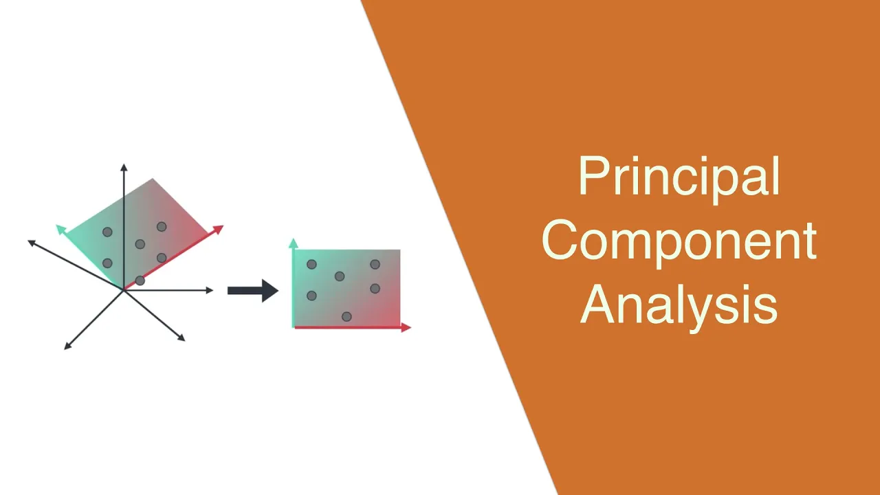

















Principal Component Analysis (PCA) is a dimensionality reduction technique that transforms high-dimensional data into fewer dimensions by finding orthogonal principal components (PCs) that capture the maximum variance in the data; the first PC (PC1) is found by rotating a line through the origin to maximize the sum of squared distances from projected points to the origin, representing a linear combination of variables weighted by loading scores, and subsequent PCs are found by finding perpendicular lines through the origin; the explained variation for each PC is measured by its eigenvalue, allowing researchers to determine how many PCs are needed to capture most of the data's structure and create interpretable 2D/3D visualizations.
Principal Component Analysis (PCA) Step-by-Step | StatQuest
Added:Basic Linear Algebra: Understanding vectors, matrices, matrix multiplication, and transpose operations.
Statistical Foundations: Grasping the concepts of mean, variance, covariance, and how a covariance matrix represents data spread.
Geometric Data Representation: Understanding how data points are plotted in multi-dimensional space and the concept of coordinate systems.
Model Selection and Explained Variance: Learning how to use Scree Plots and Cumulative Explained Variance to determine the optimal number of principal components to retain.
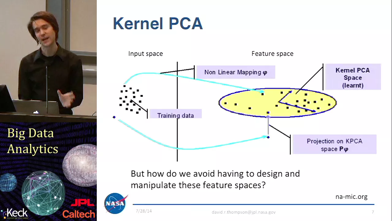
Non-Linear Dimensionality Reduction: Exploring advanced techniques like Kernel PCA, t-SNE, and UMAP for visualization and complex dataset structures.
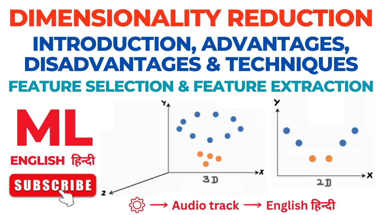
Dimensionality Reduction in ML Pipelines: Applying PCA as a preprocessing step to prevent overfitting, mitigate multicollinearity, and speed up training in machine learning models.
Singular Value Decomposition (SVD): Diving deeper into the mathematical mechanics of SVD and its application in image compression and recommendation systems.
3.5M views69.5Klikes21:57Original Release: 2018-04-02
StatQuest breaks it down into bite-sized pieces, hooray!
Hello, I'm Josh Starmer and welcome to StatQuest. In this StatQuest we're going to go through Principal Component Analysis (PCA) one step at a time using Singular Value Decomposition (SVD).
You'll learn about what PCA does, how it does it, and how to use it to get deeper insight into your data.
Let's start with a simple data set.
We've measured the transcription of two genes, Gene 1 and Gene 2, in 6 different mice.
Note: If you're not into mice and genes, think of the mice as individual samples and the genes as variables that we measure for each sample.
For example, the samples could be students in high school and the variables could be test scores in math and reading, or the samples could be businesses and the variables could be market capitalization and the number of employees.
Okay, now we're back to mice and genes, because I'm a geneticist and I work in a genetics department.
If we only measure one gene we can plot the data on a number line.
Mice 1, 2, and 3 have relatively high values and mice 4, 5, and 6 have relatively low values.
Even though it's a simple graph, it shows us that mice 1, 2, and 3 are more similar to each other than they are to mice 4, 5, and 6.
If we measured 2 genes, then we can plot the data on a two-dimensional X-Y graph.
Gene 1 is the x-axis and spans one of the two dimensions in this graph.
Gene 2 is the y-axis and spans the other dimension.
We can see that mice 1, 2, and 3 cluster on the right side and mice 4, 5, and 6 cluster on the lower left hand side.
If we measured three genes, we would add another axis to the graph and make it look 3D, i.e. 3-dimensional.
The smaller dots have larger values for Gene 3 and are further away.
The larger dots have smaller values for Gene 3 and are closer.
If we measured 4 genes, however, we can no longer plot the data. 4 genes require 4 dimensions. So we're going to talk about how PCA can take 4 or more gene measurements, and thus 4 or more dimensions of data, and make a 2-dimensional PCA plot.
This plot will show us that similar mice cluster together.
We'll also talk about how PCA can tell us which gene, or variable, is the most valuable for clustering the data.
For example PCA might tell us that Gene 3 is responsible for separating samples along the x-axis.
Lastly, we'll talk about how PCA can tell us how accurate the 2D graph is.
To understand what PCA does and how it works, let's go back to the data set that only had 2 genes.
We'll start by plotting the data. Then we'll calculate the average measurement for Gene 1, and the average measurement for Gene 2.
With the average values, we can calculate the center of the data.
From this point on, we'll focus on what happens in the graph - we no longer need the original data.
Now, we'll shift the data so that the center is on top of the origin in the graph.
Note: Shifting the data did not change how the data points are positioned relative to each other.
This point is still the highest one, and this is still the rightmost point, etc. Now that the data are centered on the origin, we can try to fit a line to it.
To do this, we start by drawing a random line that goes through the origin.
Then we rotate the line until it fits the data as well as it can, given that it has to go through the origin.
Ultimately, this line fits best.
But I'm getting ahead of myself, first we need to talk about how PCA decides if a fit is good or not.
So, let's go back to the original random line that goes through the origin.
To quantify how good this line fits the data, PCA projects the data onto it and then it can either measure the distances from the data to the line and try to find the line that minimizes those distances, or it can try to find the line that maximizes the distances from the projected points to the origin.
If those options don't seem equivalent to you, we can build intuition by looking at how these distances shrink when the line fits better, while these distances get larger when the line fits better.
Now, to understand what is going on in a mathematical way, let's just consider one data point.
This point is fixed and so is its distance from the origin.
In other words, the distance from the point to the origin doesn't change when the red dotted line rotates.
When we project the point onto the line, we get a right angle between the black dotted line and the red dotted line. That means that if we label the sides like this: A, B, and C, then we can use the Pythagorean theorem to show how B and C are inversely related.
Since A, and thus A squared, doesn't change if B gets bigger then C must get smaller.
Likewise, if C gets bigger then B must get smaller.
Thus, PCA can either minimize the distance to the line, or maximize the distance from the projected point to the origin.
The reason I'm making such a fuss about this is that, intuitively, it makes sense to minimize B and the distance from the point to the line, but it's actually easier to calculate C, the distance from the projected point to the origin, so PCA finds the best fitting line by maximizing the sum of the squared distances from the projected points to the origin.
So, for this line, PCA projects the data onto it and then measures the distance from this point to the origin, let's call it D1.
Note: I'm going to keep track of the distances we measure up here.
And then PCA measures the distance from this point to the origin, we'll call that D2.
Then it measures D3, D4, D5, and D6.
Here are all six distances that we measured.
The next thing we do is square all of them.
The distances are squared so that negative values don't cancel out positive values.
Then we sum up all these squared distances, and that equals the sum of the squared distances.
For short we'll call this SS distances, for sum of squared distances.
Now we rotate the line, project the data onto the line, and then sum up the squared distances from the projected points to the origin. And we repeat until we end up with the line with the largest sum of squared distances between the projected points and the origin.
Ultimately, we end up with this line.
It has the largest sum of squared distances.
This line is called Principal Component 1, or PC1 for short.
PC1 has a slope of 0.25. In other words, for every 4 units that we go out along the Gene 1 axis, we go up 1 unit along the Gene 2 axis. That means that the data are mostly spread out along the Gene 1 axis, and only a little bit spread out along the Gene 2 axis.
One way to think about PC1 is in terms of a cocktail recipe.
To make PC1 mix four parts Gene 1 with one part Gene 2.
Pour over ice and serve!
The ratio of Gene 1 to Gene 2 tells you that Gene 1 is more important when it comes to describing how the data are spread out.
Oh no, terminology alert!
Mathematicians call this cocktail recipe a linear combination of Genes 1 and 2.
I mention this because when someone says PC1 is a linear combination of variables, this is what they're talking about. It's no big deal.
The recipe for PC1, going over 4 and up 1 gets us to this point.
We can solve for the length of the red line using the Pythagorean theorem, the old A squared equals B squared plus C squared.
Plugging in the numbers gives us A equals 4.12.
So the length of the red line is 4.12.
When you do PCA with SVD, the recipe for PC1 is scaled so that this length equals 1.
All we have to do to scale the triangle so that the red line is 1 unit long is to divide each side by 4.12.
For those of you keeping score, here's the math worked out that shows that all we need to do is divide all 3 sides by 4.12.
Here are the scaled values.
The new values change our recipe, but the ratio is the same.
We still use four times as much Gene 1 as Gene 2.
So now we are back to looking at the data, the best fitting line, and the unit vector that we just calculated.
Oh no, another terminology alert!
This 1 unit long vector, consisting of 0.97 parts Gene 1 and 0.242 parts Gene 2, is called the Singular Vector, or the Eigenvector for PC1, and the proportions of each gene are called loading scores.
Also while I'm at it, PCA calls the average of the sums of the squared distances for the best fit line the Eigenvalue for PC1. And the square root of the sums of the squared distances is called the Singular Value for PC1.
Bam! That's a lot of terminology.
Now that we've got PC1 all figured out let's work on PC2. Because this is only a two-dimensional graph, PC2 is simply the line through the origin that is perpendicular to PC1 without any further optimization that has to be done. And this means that the recipe for PC2 is -1 parts Gene 1 to 4 parts Gene 2.
If we scale everything so that we get a unit vector, the recipe is -0.242 parts Gene 1 and 0.97 parts Gene 2.
This is the singular vector for PC2 or the eigenvector for PC2. These are the loading scores for PC2, they tell us that, in terms of how the values are projected onto PC2, Gene 2 is 4 times as important as Gene 1.
Lastly the eigenvalue for PC2 is the average of the sum of the squares of the distances between the projected points and the origin. Hooray! We've worked out PC1 and PC2!
To draw the final PCA plot, we simply rotate everything so that PC1 is horizontal.
Then we use the projected points to find where the samples go in the PCA plot. For example, these projected points correspond to sample 6, so sample 6 goes here. Sample 2 goes here. And Sample 1 goes here. Etc. Double bam! That's how PCA is done using singular value decomposition. Okay, one last thing before we dive into a slightly more complicated example. Remember the eigenvalues?
We got those by projecting the data onto the principal components, measuring the distances to the origin, then squaring and adding them together. Well, if you're familiar with the equation for variation, you will notice that eigenvalues are just measures of variation. For the sake of this example imagine that the variation for PC1 equals 15 and the variation for PC2 equals 3. That means that the total variation around both PCS is 15 plus 3 equals 18.
And that means PC1 accounts for 15 divided by 18 equals 0.83 or 83% of the total variation around the PCs. PC2 accounts for 3 divided by 18 equals 17% of the total variation around the PCs. Oh no another terminology alert! A scree plot is a graphical representation of the percentages of variation that each PC accounts for. We'll talk more about scree plots later. Bam. Okay, now let's quickly go through a slightly more complicated example. PCA with 3 variables, in this case that means 3 genes, is pretty much the same as 2 variables. You center the data. You then find the best fitting line that goes through the origin. Just like before, the best fitting line is PC1. But the recipe for PC1 now has 3 ingredients. In this case Gene 3 is the most important ingredient for PC1. You then find PC2, the next best fitting line given that it goes through the origin and is perpendicular to PC1. Here's the recipe for PC2. In this case Gene 1 is the most important ingredient for PC2. Lastly, we find PC3, the best fitting line that goes through the origin and is perpendicular PC1 and PC2. If we had more genes, we just keep on finding more and more principal components by adding perpendicular lines and rotating them. In theory, there is 1 per gene or variable, but in practice the number of PCs is either the number of variables or the number of samples, whichever is smaller. If this is confusing, don't sweat it. It's not super important and I'm going to make a separate video on this topic in the next week. Once you have all the principal components figured out you can use the eigenvalues, i.e. the sums of squares of the distances, to determine the proportion of variation that each PC accounts for. In this case, PC1 accounts for 79% of the variation, PC2 accounts for 15% of the variation and PC3 accounts for 6% of the variation. Here's the scree plot. PC1 and PC2 account for the vast majority of the variation. That means that a 2D graph, using just PC1 and PC2, would be a good approximation of this 3D graph, since it would account for 94% of the variation in the data. To convert the 3D graph into a two-dimensional PCA graph, we just strip away everything but the data and PC1 and PC2, then project the samples onto PC1 and PC2. Then we rotate so that PC1 is horizontal and PC2 is vertical. This just makes it easier to look at. Since these projected points correspond to sample 4, this is where sample 4 goes in our new PCA plot. etc. etc. etc. Double bam! To review, we started with an awkward 3D graph that was kind of hard to read, then we calculated the principal components, then, with the eigenvalues for PC1 and PC2, we determined that a 2D graph would still be very informative. Lastly, we used PC1 and PC2 to draw a two-dimensional graph with the data. If we measured 4 genes per mouse, we would not be able to draw a 4-dimensional graph of the data, but that doesn't stop us from doing the PCA math, which doesn't care if we can draw a picture of it or not, and looking at the scree plot. In this case, PC1 and PC2 account for 90% of the variation, so we can just use those to draw a 2-dimensional PCA graph. So we project the samples onto the first 2 PCs. These 2 projected points correspond to sample 2, so sample 2 goes here. Bam! Note, if the scree plot looked like this, where PC3 and PC4 account for a substantial amount of variation, then just using the first two PCs would not create a very accurate representation of the data. However, even a noisy PCA plot like this can be used to identify clusters of data. These samples are still more similar to each other than they are to the other samples. Little bam. Hooray! We've made it to the end of another exciting StatQuest.
If you liked this StatQuest and want to see more, please subscribe. And if you want to support StatQuest, please consider buying one or two of my original songs, the link to my bandcamp page is in the lower right corner and in the description below. All right until next time quest on!
Up Next

28:55
Singular Value Decomposition (SVD) Explained | Matrix & Image Compression
@SerranoAcademy
107.1K views•2020-09-08

4:43
Elliptic Curve Cryptography Explained: ECC, ECDSA, ECDH
@PracticalNetworking
28.5K views•2024-10-21

16:14
Mutual Information Explained: A Clear Step-by-Step Guide
@statquest
164.6K views•2023-02-06

6:00
The Mathematical Impossibility of Accurate World Maps
@Vox
23.3M views•2016-12-02
Related Study Plans & Knowledge Roadmaps
Structured learning paths in Mathematics
mathematics
Tensor Calculus: Vectors to Riemann Curvature
01Mathematical Foundations: Linear Algebra & Calculus
02Covectors, Dual Spaces, and Tensor Basics
03The Metric Tensor and Index Gymnastics
+ 2 more learning modules
40h5 modules
Explore Roadmap
mathematics
Gödel's Incompleteness: Logic, Proofs & Limits
01Introduction to Formal Systems & Hilbert's Dream
02Set Theory, Cardinality, and Cantor's Diagonal Argument
03Arithmetization and Gödel Numbering
+ 2 more learning modules
14h5 modules
Explore Roadmap
mathematics
Galois Theory: Fields, Groups & Solvability
01Foundations of Abstract Algebra: Groups & Fields
02Polynomials & Field Extensions
03Splitting Fields & Symmetries
+ 2 more learning modules
24h5 modules
Explore Roadmap
mathematics
Non-Euclidean Geometry: Models & Geodesics
01Euclid's Fifth Postulate and the Birth of New Geometries
02Hyperbolic Space and the Poincaré Disk Model
03Geodesics: Defining Straight Lines in Curved Spaces
+ 2 more learning modules
15h5 modules
Explore Roadmap