







![[53a] Intro to PyTorch Tutorial (Sebastian Raschka)](https://i.ytimg.com/vi/B5GHmm3KN2A/maxresdefault.jpg)






![[DL] The convolution operation](https://i.ytimg.com/vi/wjfxPotXV1U/maxresdefault.jpg)





![[M2L 2024] Graph Neural Networks - Helena Andres](https://i.ytimg.com/vi/4FQABJQVWkI/maxresdefault.jpg)


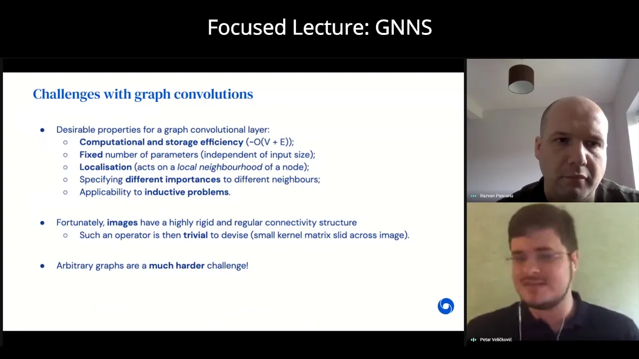
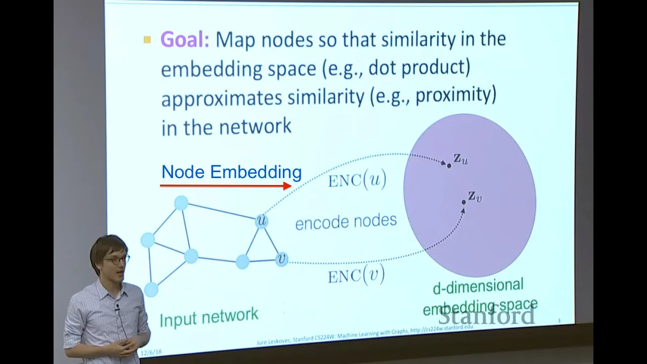
Geometric Deep Learning extends traditional deep learning to non-Euclidean domains like graphs by using computation graphs where each node aggregates information from its neighbors through order-invariant operations (such as mean or max pooling), allowing models to learn node representations that can be used for classification, regression, or other tasks on graph-structured data.
Geometric Deep Learning with PyTorch Geometric: An Introduction
Added:Proficiency in Python programming and familiarity with standard machine learning workflows.
Basic knowledge of PyTorch, including tensor operations, model definition, and the training loop.
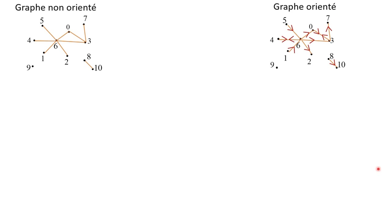
Fundamental concepts of Graph Theory, such as vertices (nodes), edges, adjacency matrices, and directed versus undirected graphs.
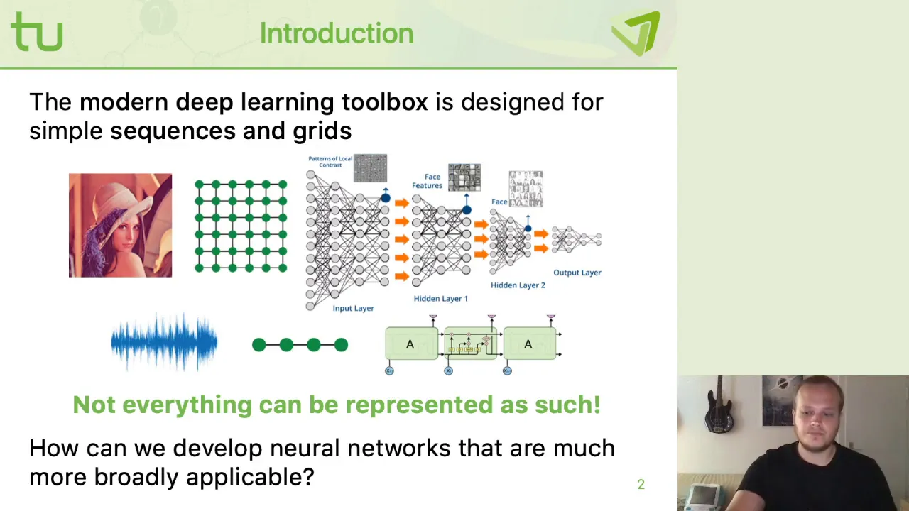
Core deep learning concepts, specifically how convolutional layers extract features from structured grid data.
Advanced GNN architectures, including Graph Attention Networks (GAT), GraphSAGE, and Message Passing Neural Networks (MPNNs).
Scaling Graph Neural Networks to large datasets using neighborhood sampling and mini-batching techniques in PyTorch Geometric.
Designing custom message-passing layers by overriding PyTorch Geometric's base MessagePassing class.
Practical applications of GNNs, such as molecular property prediction (chem-informatics), social network analysis, and recommender systems.
76.7K views1Klikes47:44Original Release: 2021-02-17
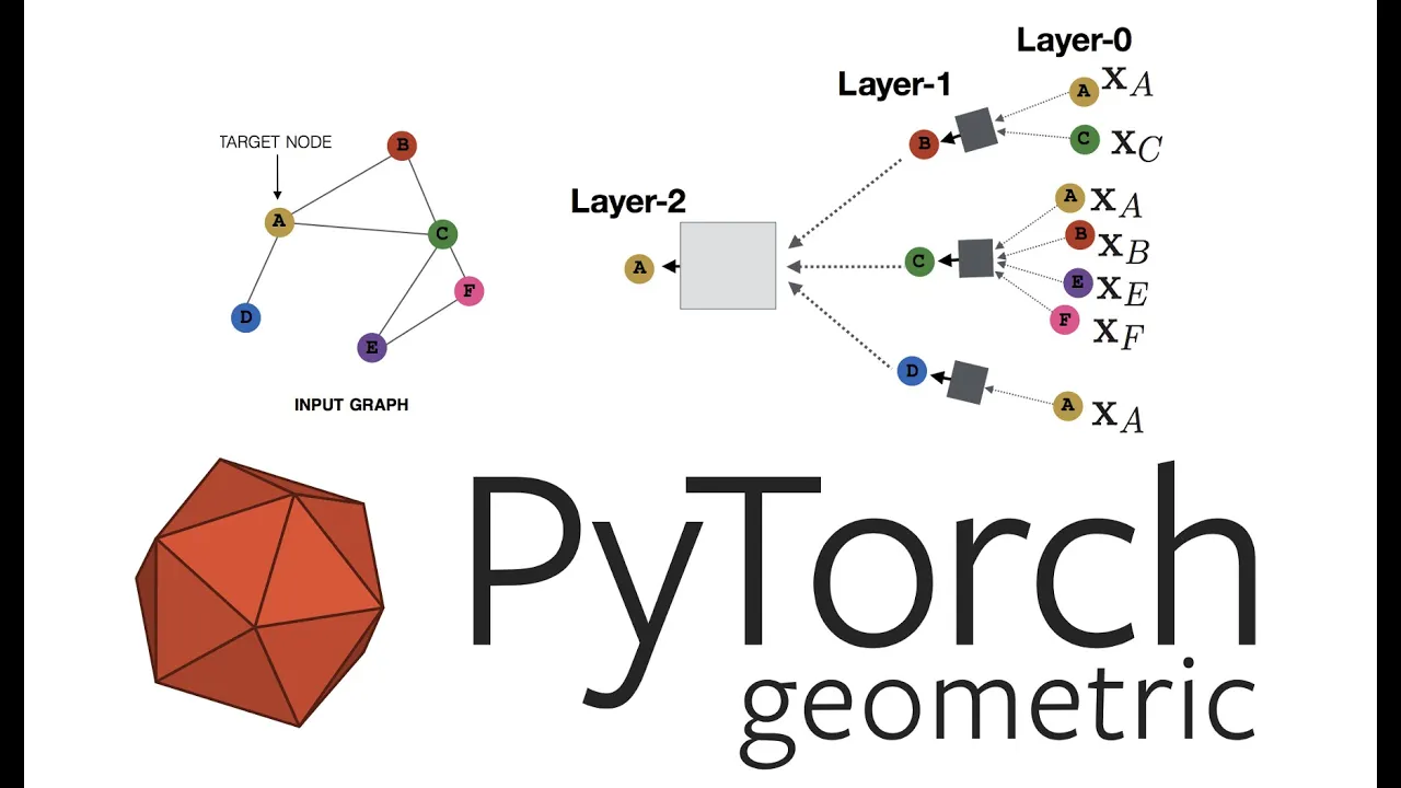
good morning to everyone i am antonio longa and i'm here to present uh this journey that uh me and gabriel essentine decided to start the the idea is that uh nowadays geometric deep learning is is becoming uh really useful in many areas and we make some trouble we have actually we had some trouble finding a material and easy to use code so the idea is to [Music] start this this yeah this journey together and the idea is that we will have every weekend uh weekly meeting and we will discuss about uh geometric deep learning and present something today we are gonna um see something really really basic and just an introduction the biggest part of this tutorial will be theoretical and then we will see something related to the implementation so uh let me share my screen and i preferred some slide and okay the title of the presentation of today is what is geometric deep learning and just present this okay uh as i said we are antonio longa and the gabriele santine this is an open source project meaning that everyone can use our code have a look on youtube on on our videos and the idea is to learn how to use geometric deep learning um we will use the framework pytorch geometric that has been released a few years ago so it's quite new how it works we will have a brief introduction to our geometric deep learning model and then we will apply the the model which is presented and the idea is to uh keep uh update with the news and if you i don't know if you find an interesting model and you want to present it just feel free to join us ask and present whatever you want who are you the idea is that you can be a student a researcher an engineer whatever you want and it's obviously totally free and you can join us and follow everything just to say uh we have an official website that is uh geometric deep learning tutorial uh i touch dramatic tutorial and here we will see for every lecture a new post and with a brief summary and finally we will find the video on youtube the link to the video to youtube and also the repository on github containing the material the slides and the jupiter notebook okay let's start okay where we were we were here okay today we are gonna see uh deep learning and uh which are the fields of deep learning then we are gonna talk about graph and graphs representation and some deep learning and deep learning problems in terms of graphs and deep learning some definition graph neural networks and a little bit of practice let's start as you probably probably know deep learning is uh has been in the last decades has been used in several areas like image medical images speech recognition uh and in the last decades we achieved the amazing results uh throw the deep learning techniques on these fields but what about other fields like biology the recommendation system network science or main food uh well what what which is the difference the main difference between an image and a manifold or a speech and a molecule an error x image and a graph well the latest state on non equilibrium domains and talking about the graphs we have several type of graphs like uh directed graph uh node labeled oops node labeled graphs undirected graph edge labeled graphs so as you can see this kind of structure as an a specific structure and can cannot be modeled as an image that is that basically is a grid of pixel or a speech that can be seen as a chain of information and talking about the graph representation a graph can be as you probably know a graph can be represented with an audio synthesis matrixes what does it mean it means that if the graph has i don't know sixth note like in this example we have these matrices six by six six times six in which the element uh in position aj is zero is one if there is an arch in the graph and it's it's zero otherwise in such a case uh we have an undirected graph so the at the end of this matrix is symmetric uh okay but uh if we have these matrices these uh well structured the squared matrixes why we cannot use neural networks i mean uh an image we say that it's a square is a matrix and which is the difference between a matrix and i mean an image and an audio synthesis matrixes and why we cannot give us an input our audio synthesis matrix to our neural network even convolution if we think about convolution well basically the idea is to uh make inference on uh i mean on a little size of the image and make a convolution on on that part we could do the same in a graph we have these matrices and we can took small portion of the image a compute something uh some convolution and well the work is done we haven't finished it and the course is finished unfortunately doesn't work because uh this is not a good idea actually is a terrible idea because what happened if a new edge pop in the in the graph so what happened we if we have different sizes of graphs and another big problem is that the metrics representing a graph that's idea synthesis matrix is not invariant to node ordering so what does it mean different size simply as i introduced you suppose that this new node g appears on the graph and then uh so also the idea synthesis matrixes will be bigger like in the sphere and if we train at our model to this first neural network then we will need a new input uh a new input uh a new input etc and the network is not trained to do this so this is a problem another problem uh is that uh the idea synthesis matrix is not invariant to not ordering what does it mean if we have these two graphs as you can see the only difference of these two graphs are the node ordering i mean the name that i give to the nodes but the graphs are isomorphic in fact g is equal to g prime but if we have a look to the idea sentences matrixes the idea synthesis matrix of g and g prime are totally different even if the graph is identical and this is why we cannot use the simple geometric the simple deep the simple well the well-known deep learning on images we cannot use it for graphs and as i said the motivation now is obvious not in not invariant to node ordering a and also um its different size make create huge problems okay just a really brief definition we have a graph uh like this one that is defined as a as a pair of vertices and edges and we have the representation of this graph structure analysis sentences matrixes and moreover i mean we also have um um a feature vect of a feature metrics another feature matrix is that is a matrixes as as you can see the number of rows is equal to the number of nodes in the graph while the number of columns is equal to the feature the number of a feature on each node and we just have this additional information on the graph so uh from now to the end we will use g as a general graph a as a synthesis matrix of the graph and x as the node feature then matrix containing the node features of the graph okay we are going to present the graph neural networks first of all we have to define what's so-called computation graph and then we are gonna use the computation graph to infer something from the graph okay what is the computational graph the computation graph is the neighbor of a node define its computation graph what does it mean just took this example we want to make some inference on the node a the red node in the slide we just took the node a and we up these boxes and this box i will tell you what this boxes is later then we took the the second node the node connected to a and then we connect again these boxes and we connect all the nodes connected to f what does it mean we have b a and e connected to these boxes that goes inside f that goes inside this new box and goes to a what does it mean it means that we have the feature vector the node feature of the node a the feature of the node b and the feature of the node e such information information goes inside this box in some way they are combined with the feature of the node f and they goes inside the node a uh yeah just this just was a was i was saying that uh okay here we have the the representation of uh the yeah they know the feature of a b and e what those boxes are well they are neural networks and what is inside this operation i mean what we can do with the representation of a b and e we have to do an aggregation in particular we have to do an order invariant of a aggregation like for instance the sum is ordering variant the average is ordering variant because doesn't matter if we add the abe or if we add the bae this the result uh will be the same and it's important to have an aggregator that is ordering invariant okay every node defines its own computation graph so for instance you already saw this computation graph for the node a for the node b as you can see at the first step we have three different nodes f e and c and here you can see a e f c and then the neighborhood again for instance uh from f we have a and e and b so we have a b and e from c we have e and b and a b and h and so on in uh the same for c d e and f and so we have this uh computation graph for each node in the network okay can you see some redundancy yes of course for instance uh this part in which the node f is involved on the representation of a we have here the same here the same here the same and it's equal for b c every node as you can see are they are repeated okay in terms of neural network what we have we have the layer 0 in which we have the representation of the uh the node feature the layer 1 in which we have some kind of hidden layer and when and then we have our last layer in this little example well a question is how much you have to unroll well suppose that you want to make some inference to that node the red node in the graph well if i unroll one time i will arrive here two times i will write here and one question is when i have to stop unrolling this this information well in terms of for instance social network probably in order to infer something about me probably is not necessary to took information also from a guy living in boston who i never never met and i not even know who he is but maybe my friends know something about me the friends of my friends know something about me it's also important to think about the diameter of the network because if you on a roll too much then you are seeing for every node you are collecting information from all the network and that well probably is not useful for it okay let's start with a little bit of math so uh okay we have that the etch each represent the representation of the node v in the layer in the layer 0 well the representation of node v at layer 0 is the node v itself what does it mean in our previous example where we had this vector of three integer integers as a node feature in the first in in the layer 0 we have that the representation of the node is just the feature vector then what we have we have some computation in which we have that know the the embed the representation of node v in the layer clay k plus 1 is equal to something and finally we are gonna we we can see that the representation of node v uh we call actually we call the embedding of v z of v is equal to the last layer so the k layer of the northern v okay now we want to look inside this uh creation is just the copy of this middle uh this middle uh equation yeah okay let's start uh we already said that this is the is the k plus one embedding representation of the node v it's a lattice representation then we have this is equal to the embedding of node v advocate embedding so what does it mean my embedding in this in the next layer is equal to my embedding in the previous layer so we have just h of v at the gate level okay and then we have this operation for each uh that basically is the average of the previous embedding of the previous representation the presentation in the previous layer of every neighborhood of the node v okay then what what we have we have two waves w and b associated to this layer and finally we have an activation function a non-linearity for instance and as you can see here we have a summation okay here we have a mean about all the neighborhood of the node of the current node we have some trainable waves and we have again trainer wall waits in my previous embedding and we just summit uh passed through an activation function and we have the representation of the k plus one layer as you can imagine uh all these structures uh share this the parameters wk and bk and it's the same for each element in the network i mean not for each element sorry for each uh computation graph we have this parameter are shared together because because it allows to when a new node arrived or a node that we didn't use for training but we want to use for testing we are able to be what we call the previously unroll and build the computation graph then we have the already trained waves w and k for each layer sorry w and b for each layer and we can propagate the information and produce the embedding of node e okay um we are close to go to the practice side uh i want just to talk about gruff sager because is really really uh an easy modification of what we did so far and moreover it allows us to give um representation uh sorry ah already build a function on pytorch so we can see in practice what does it mean okay we have sage is a work done by william hamilton in 2018 and uh okay these three equations are the same we saw previously okay which is the difference with respect to uh this new paper well they change only this middle equation the the the equation for the middle the the hidden layers and what they do well instead of using the average here they use a general aggregation okay and it's the same here we have aggregation here we have a min and as you can see for every neighborhood every node in the neighborhood of the node b and above is the same for every node in the neighborhood of the node b uh instead of doing the mean we do something else that we will see and another modification that they do actually they did was to instead of summing the information given by myself in the previous layer so bk and multiplied by h vk instead to sum together this information so uh as i said the information came from my neighborhood and the information came from myself instead of do this uh hamilton decided to concatenate this information okay so as you can see here is just a concatenation in fact as you can see here we have the first part the change so a general aggregation function and then we have from a plus we we we go to a comma meaning a concatenation okay what this aggregation is well it can be a pulling strategy uh like element wise mean max or whatever you want or also even uh lstm note that an lstm uh or we will see uh everything of these in the next uh tutorial not today but just to say something note that lstm is not ordering invariant however uh there are some there is actually there are some works that answered that if you compute lstm several times with a random permutation of the input you can achieve quite good results but i don't want to talk about these because this is just an introduction okay i think we have done i i presented the general idea and now i want to show you a really really simple example in a way that you can try this at home uh okay okay uh let's start uh simply at the beginning we just import uh torch geometric and we are gonna use uh uh already defined um data set so we are not to use our own data set but we are going to download it from from torch geometry and in particular it's uh really simple uh we give a name of the data set we call the this this uh function and then we set a root meaning that it will create a folder uh with all the the file suppose that i'm gonna delete this folder and we are gonna run it what happened it start downloading from internet the data set and then build it as you can see here uh geometry uh torch geometric build this folder containing the raw file so this core data set in a raw file fashion and also the proceed file what does it mean it means that if already i have this data set and the next time i'm gonna i don't know uh suppose restart the cabinet and clear output okay and run again you can see uh pytorch geometric can see um that the file is already in the downloaded and that it just loaded without any uh download again okay what about the dataset properties data set in our case is cora that is a citation graph in which is a rough representing different paper and how they are cited among them so as you can see here if we print the data set we can see its name is cora and uh and then if we look at the length of the data set is one because we have just one graph on a huge graph we also have this property number of classes we have seven different classes we have node feature so in particular each node has a 1433 feature and also we have zero edge feature you can see all this information only with exceeding the the property of the data set the data set also have the data the data we are gonna use in particular uh the graph is represented as a edge index so uh simply have a look here in the the first print the edge index as sides as a shape of two multiplied by this number here that's the same here as as you can see uh as you can see here we have the node zeros goes in the node 6 33 you not zero goes and so on we also have a training mask a test mask and a validation mask those are a vector as you can see i i mean one dimensional tensor and we have boolean values representing which nodes are on the train set on the test set and on the validation set uh we also have x x is the node feature as i said to you is quite huge we have 1433 feature for node in fact the shape of the x is the number of nodes multiplied by the number of node feature and here is just an example finally we have why why is the node labeling the node the uh yeah the node labeling so every node belongs to a different category for instance the node zero belong to category three the node one belongs to category four and so on so forth okay here we took the data load the data uh without actually in the next lecture we will see how to uh load your own graph your own data set we will see function that allow you to convert from networkx to by torch from by torch network x and several others function okay here we are importing again torch torch functional as f uh they came from the original library the torch library and then we are import sage conf that is the the last uh slide i show you uh from torch geometric here we are gonna say that the data is that set in position zero because we have only one data set what we are going to do here we are here we are going to define our neural network uh easily is uh is is kind of standard we define this class he never date from torch and then module we can use init define the init function that is uh called super itself and call the init function but don't be scared about this because we will this is just an easy example to show you how it's easy to run it but we are not gonna we are not gonna cover the details of this implementation we will see it in the next lecture but this is just the beginning and i want to introduce you to the framework and see and show you how can you use it so we were here we just defined this self conv whoops we call the uh convolutional layer we just imported and we with the the the convolution layer require an input channel and an output channel and what we did we do actually we just do a data set the number of feature so meaning that this input is huge is uh this number here and the output is the number of classes so seven as you can imagine this is not going to work very well because we are passing from directly from 1000 and so on to for feature we can specify the aggregation the uh aggregation we want to use and for instance i decided to use the max okay and this is just the initialization of the network then we have the forward so we just define that the x is equal to the uh convolution so a function defined here and with passing input the data and the edge index that is uh what it's required to run and finally we return the log softmax of the function don't worry about this and and else but we are gonna talk uh with everything in details don't worry here uh we can use uh okay what does this function do well this function allows us to decide if to uh put our uh model on the cpu or in on the gpu for instance uh in my pc i have enabled and installed all the libraries for cuda so my device is called up because it's available and what happened that we move our model so our network and also our data to the gpu but don't worry really we are gonna cover it uh we have an optimizer and whom is uh already know about uh machine learning probably already know this optimizer is adam taking input the parameters of the model he has a learning rate away decay but we will cover with more time and much more details this stuff and then we have two simple functions one for the train in which we train our model and one for the test and i'm not gonna spend time here on this simple to function because we will cover it as i said and then we are gonna just to run it for 100 ebooks and see the results okay we here we have the validation on in the test in accuracy yes the validation and the test accuracy in with this toy example as you can see there is no improvement uh quite the quite stable we did the few epochs but who cares because really the model is really really simple we don't have dropout we don't have linear layers we don't have almost anything and that's all i i really wanted just to show you the basics and introduce you to me and present this idea to i don't know work together and learn together uh by torch jamith does anyone has any question i have a question actually so first of all thank you uh very great introduction so i'm almost new uh to uh twins library pie torch and i also got a small connection problem at the very beginning so i don't know if you already covered it so i was curious about the uh let's say problems uh uh in the sense of uh classification regression and so on that you can take luxury with this uh uh geometric uh neural networks in the sense that you presented the uh like a classification of nodes right oh is there anything else that you you can do yeah of course uh because let me share my screen okay here uh okay here when we have this uh okay this one is really really simple but when we have this we can also instead of using softmax we can use uh actually what we have is uh not the embedding representation we have a learned representation for each node and then we can use such representation for everything regression whatever you want because uh what you have learned so far is an old representation okay okay great so you can also do stuff with the edges like classify edges okay okay great well actually is well we are gonna cover this definitely because i think it's interesting but basically what we are what you do if you have uh if you want to do something related to edges well instead of building this computation graph you build it is in terms of couples for instance the edge between a and f appears here and the neighbor had just instead of having notes you have representation of edges okay okay thank you okay something uh someone else i have one kill you as a team you showed us uh the interesting framework in which from each note you basically collect information from its neighborhood means neighbors and then you you might enroll the network as much as you want my questions concern my question concern the case in which you have for example self loops what what does happens if you have certain loops so you're basically feeding your hidden layer with the let's say information from the node then you're basically it's let's say it's the level zero of what should happen when you unroll too much that you are i don't know it's a kind of overfitting or or what is it well i i think you can handle in different ways for instance uh if you think about the math we saw just so we still have the representation of our self but you can even think to remove some self loop or limitate them after a while you see what i mean i mean instead of uh heat cycling on itself you can do this up to a given time then stop it yeah so basically you're treating uh self-loops let's say uh self-edges as a different type of yeah connection from there yeah but i i'm sure that someone someone has already uh tackled this problem but i saw i mean so right now i i've read nothing about it but uh interesting thanks oh it was just a curiosity i mean i don't even know if it's really overfitting or what what what is it doing so i'm just just like but thanks i think so but anyway i think we can maybe keep it to keep these in mind for a future meeting so just discuss what happens in those cases and yeah be a great idea yes yeah so something that i didn't so i'm really new also to this topic so that the the number of layers is related to the size of the of the neighborhood that you are considering right so because every time that you compute a new a new layer you are increasing the the computational graph right yeah but exactly maybe i didn't explain very well no no it was very really clear i think so you're right we have two level of that in a sense that for instance here uh we have really uh two levels of that because so far we can see that uh it seems that this competition graph is a a depth of three because first second the third well two but by the way but note that we have the depth of the computation graph and then we have the back of the network this neural network can be uh depth as much as i want i mean okay i see it so those are yeah yeah terms we have different depth different uh yeah different depth okay you see yeah because i think it's much more expensive if you have so if you increase you want a method to that is local so you don't want to consider the entire graph every time so if you have a very deep uh structure you are you need to consider very large parts of the graph every time so and the easy idea is that uh often uh in order to uh make inference about one node probably is not so important to go so wide and and deep okay okay thank you you and i hope to see you also next week and uh i think next week we are gonna see with gabrielle some basics of uh by torch so what we saw today but uh in a more specific way and in by torch not in fire torch to matric and then we are going to move to white thank you guys thank you thank you thank you
Up Next

54:56
Graph Data Handling in PyTorch Geometric | Part 1 Tutorial
@94longa2112
19.7K views•2021-05-25

87:26
Introduction to Secure Multiparty Computation with Yehuda Lindell
@fhe_org
7.7K views•2021-02-04

41:36
PyTorch Basics for Graph Learning: Datasets, Models, Losses, Optimizers
@94longa2112
20.7K views•2021-02-23

19:25
Enigma Machine Mechanics: WWII Encryption Explained
@JaredOwen
13.2M views•2021-12-11
Related Study Plans & Knowledge Roadmaps
Structured learning paths in Computer Science
computer-science
Container Runtimes: Namespaces, Cgroups & Go
01Linux Systems & Go Programming Foundations
02The Core of Isolation: Chroot and Filesystems
03Linux Namespaces: Process Isolation
+ 3 more learning modules
32h6 modules
Explore Roadmap
computer-science
Building a CHIP-8 Emulator: Rust & CPU Basics
01Computer Architecture Foundations (Bits & Bytes)
02Rust Programming for Systems Development
03CHIP-8 Virtual Hardware Specifications
+ 2 more learning modules
32h5 modules
Explore Roadmap
computer-science
Building BitTorrent: Go, P2P & Concurrency
01Go Fundamentals & Concurrency
02Networking Foundations & P2P Architecture
03Bencode Parsing & Torrent Metadata
+ 3 more learning modules
26h6 modules
Explore Roadmap
computer-science
Actor Models (C++ Concurrency & Lock-Free)
01C++ Multi-Threading Foundations
02Thread Pools and Task Scheduling
03Atomics and Lock-Free Queue Design
+ 3 more learning modules
45h6 modules
Explore Roadmap