
















![Heterogeneous graph learning [Advanced PyTorch Geometric Tutorial 4]](https://i.ytimg.com/vi/qL09oshDKww/maxresdefault.jpg)




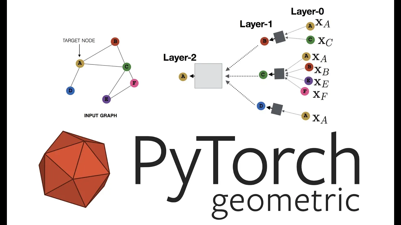
PyTorch Geometric provides structured classes for graph data handling: the Data class represents a single graph with node features (x), edge connections (edge_index), and optional attributes; the Batch class extends Data to handle collections of disconnected graphs; the NeighborSampler enables efficient neighborhood sampling for large graphs; and the Dataset class provides pre-configured datasets with built-in transformations. The library supports four main graph learning tasks: node prediction, graph prediction, edge prediction, and link prediction, each utilizing node embeddings refined through graph convolutional networks followed by readout functions.
Graph Data Handling in PyTorch Geometric | Part 1 Tutorial
Added:Basic proficiency in Python programming and Object-Oriented Programming (OOP) principles.
Solid understanding of the PyTorch framework, including tensors, datasets, dataloaders, and basic neural network training loops.
Fundamental concepts of Graph Theory, such as nodes, edges, directed/undirected graphs, and adjacency matrices.
Conceptual awareness of Graph Neural Networks (GNNs) and how graph data differs from standard grid-based (image) or sequential (text) data.
Implementing and training standard GNN architectures (like GCN, GAT, and GraphSAGE) using PyTorch Geometric.
Scaling GNNs to massive graphs using advanced mini-batching techniques and scalable neighbor sampling algorithms.
Working with heterogeneous graphs in PyTorch Geometric, where nodes and edges can have different types and feature spaces.
Applying PyG data pipelines to real-world tasks such as link prediction, node classification, and graph classification.
19.7K views226likes54:56Original Release: 2021-05-25
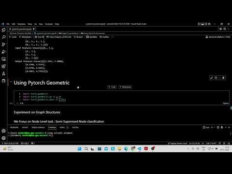
oh hello everybody uh so today's tutorial is going to be the first part of uh to a session tutorial in which we're gonna uh talk about uh how we handle data and how we can uh also uh implement uh new data sets into a pi torch geometric so today is going to be um a little bit of an overview basically of uh what are the classes and the um the data structures that are implemented in python geometric for uh handling graphs and uh batches of graphs and data and the next time it will be more about how we can implement our own graph basically so just to uh start again with our brief recap so we have had many uh tutorials now so we can say that um we identified uh four main tasks uh uh we can perform on graphs basically so the first the the four tasks are uh node prediction so predicting some property of the nodes uh graph prediction which is a predicting property of the graph edge prediction same thing uh for the edges and also uh add prediction in the sense of uh link uh connection so basically uh connection between uh predicting connections between node in the graph so uh starting from the first one so we have seen that in our prediction what we usually do is uh we start by basically having uh these embeddings of the nodes which we uh refine through uh uh whatever graph convolutional network we want to use uh for a different um depth or timestamps uh t basically if depending of uh if we are talking about rough convolutional network or graph or recurrent neural networks um in order to basically obtain uh at the end at the final iteration k uh a matrix uh of uh node uh embeddings uh from which we can then use a readout function which is usually implemented as a multi-layer perceptron in order to obtain uh our final value uh for instance uh if it's a classification binary classification problem we will we would end up with a predicted array which is the the predicted predicted class of the nodes uh this the almost the same procedure goes for the graph prediction so still uh we obtain these metrics of node embeddings at the iteration k but uh what we do in um pulling pretty in a graph prediction is uh we basically apply a pulling of a global pooling function a global operation global pooling operation which is usually a permutation invariant function uh that we apply element-wise in order to obtain a single representation of single embedding for the entire graph and then later again using a readout function we can predict the property of the graph basically the same goes for edge predictions in which we have uh the embeddings of the edges for instance we have seen how in a node to back we can obtain these embeddings by merging the embeddings of the two nodes that the the edge connects so we end up having the embeddings for the edges and then again applying a multi-layer perceptron we can obtain the prediction the fourth um task that we have seen is basically uh predicting uh the connections of two graphs so we have seen how uh how uh using a graph autoencoder we can basically uh predict a new adjacency matrix which um which will basically give us new connections uh for a given graph so this is what a lot of the four main tasks that we have seen uh in our tutorials but we have never really and we have showed a lot of uh jupiter notebooks in which we uh handle um this kind of graph data and um how we uh can basically perform these tasks but we have never talked about how we uh manage data in pythagorean metric so um let's start by defining which um which are the main modules um that pythometrics makes available for um managing and uh transforming data so basically uh in python geometric we will have uh these two sub models which are data and data sets uh so uh the data submodule contains the classes and methods uh that allows us to create and manage a single graph or a collection of graphs and also it makes available the methods to perform operations on these graphs so basically for instance how we can uh create a single graph uh data in python geometric how we can collect a batch uh create a batch of graphs uh in python geometric or for instance how we can apply a plastering uh um in the graph or uh some other basically operation whereas for instance for the torch geometric uh data sets of modules that is basically a collection already prepared collection of data sets that are available uh in the library that we can use as is uh for uh solving uh the tasks that i told you about so um i will go now a little bit back and forth from this to the jupiter notebook in order to show you uh the implementation of the classes and also um to let's say um have um to put our hands uh to work with the the actual uh code so let's start from uh the basic the most basic class that we can get which is the the data class this uh class basically represents a graph so basically uh whenever we say we see data a data object it is basically representing a graph so um this is a little bit tricky remember because a graph can be like a graph in which all the nodes are connected but also it can be that you have several graphs which are disconnected but they are still uh put in uh one um data object so basically because graphs actually can be represented also in this way so um we will see a little bit later uh what it means but let's uh for now be stuck with the data being a single graph so basically in order to initialize a data object uh we need here um some values so for instance x which is the the metrics of uh the nodes of the embeddings of the nodes in which we have on one dimension the number of nodes um that we have in the graph and uh the number of feature um for the number of dimensions of the embedding basically um then uh all the graph is also represented by uh the connections which is um given here by the edge index matrix which is a matrix uh which is composed by um two dimensions and the number of edges which is basically uh one column for one dimension sorry for uh the source um of the of the edge and uh the other for the target so basically uh from uh where the edges start and for uh to where it uh points basically then we can have also additional information like for instance the edge attributes which are uh let's say supplementary information uh that you can give to the edges of this graph also you uh we can give assign the target value to for which is why in this case to uh either the the entire graph or the notes of the graph it depends on which kind of task we're going to perform uh on a specific graph where if it is node prediction or graph prediction and then um we can have also uh other kind of information so basically um we can have how many faces if you are i mean we can have information about the faces of the graph if you are looking for instance about the mesh or um we can have um the normal uh the normalized uh matrix uh for basically uh then uh for each node of the of the graph okay so this is uh the most basic object that we can find in the for representing a graph also what we want we can do is uh we can represent collections of graphs basically so uh this we can do it with uh the batch class which extends uh data so basically a batch extends data it's a little bit tricky to think about it because usually it's the the other way around but uh batch is actually a data object but it has some other properties because it allows us to handle a collection of graphs so um in the batch uh class we have all the functions that we have seen in the data but also we have uh some other functions which are uh this one so from data to list from data list basically and to data list which is basically if i want to initialize a batch how do i do it i can just simply call this function from data list and if i give an input a list of data objects basically what this class does is it will take all the single graphs in the list and will put it all together into one single uh data object representation which is um one graph that contains all the graphs in the list but disconnected okay um batch allows us also to do the reverse so basically once we have initialized it uh this big disconnected graph with from data list we can also retrieve the single um graphs the initial single graphs using um two data lists basically we can also check how many graphs we gave an input in the list which is number of graphs and this um this is the the let's say the main object when you also use a data loader so basically a data loader gives in output a batch object okay okay so basically the the these first two uh classes are just like for the single graph representation then um there are also another coup some other classes which are very interesting to me that i want to talk about which are basically cluster data and cluster loader so basically um if you are dealing with very large graphs okay and the computation is very uh complicated because maybe uh you have uh these um these very large graphs and you don't really want to explore too much of the neighborhood of a node you can basically use the concept illustrated in this paper which is called clusters gcn which basically um what the what does it what does this algorithm do it basically takes these large graphs and tries to compute clusters in the graph and basically by computing these clusters each node is assigned to a cluster and also when you basically use the cluster loader it will be returned clusters of um of nodes basically so this is a strategy in order to um avoid uh i mean to to basically deal with very large uh graphs okay uh but uh this is okay yeah then another class that they found really interesting is the neighbor sampler which allows us basically to sample some a specific number of nodes in the neighborhood um in in a neighborhood basically uh which is basically the same concept as we have seen it in graph sage okay in graph sage you have that at a certain point you don't really use the entire neighborhood of a node but you sample uh some rules from it okay how do you how do we do it in python geometric using neighbor sampler okay so neighbor sampler is a class that basically takes an input the edges of the graph and um basically what it returns is a data structure that contains the nodes the the sample nodes and uh the sample connection okay for uh the nodes uh to note here is that um we have uh how when we initialize it we have also to specify sizes what is it so basically sizes is a list of uh integers which basically represent uh for which the the length of sizes is basically the number of convolutional layer that you're going to use in your graph neural network model and the value inside each each element of this list is going to be the number of nodes to sample for that layer basically so we will see it better uh in the in the actual implementation but um this is it then we have also that we can specify uh some nodes that um we want to consider and which one we want to avoid basically uh from the the sampling procedure so we we simply want to um for instance uh sample train nodes okay so i will give here uh an input a list the list of the indexes of the train nodes and the sampler will sample only three nodes okay um and then i mean simply the number of nodes in the graph okay so this is uh the first okay so this is the the first block of stuff that i wanted to talk about let's see uh how uh we uh can use all this stuff in the actual implementation so basically okay here i will do my import i will start basically to illustrate to you how we can use all this kind of stuff by by using a simple example so basically here i will create a dummy graph which has no meaning whatsoever it's just for uh illustrate illustration purpose uh but i think it really um will help you to understand what to uh um what these classes basically do so here i will start uh by creating the embedding the metrics embedding of the notes so here uh what i'm gonna do is uh i'm gonna have a graph for which we have 100 nodes and the the the length of the embedding of the node is going to be 16. so we are we're going to have 16 dimensions for um for each node okay uh i simply generated right now because i don't really i'm not really interested in the actual values okay can i talk to you can i ask you something yeah sure of course what you call embedding are the node features right uh yes basically okay so that is there is a given embedding it's not that we are trying to build other building no no no yeah okay maybe this is misleading but it is actually the initial node features okay perfect thank you for the introduction so um okay so now we have uh our uh yeah and calling them addings is a little bit misleading so we have our node features uh let's create the connections of the graph so basically uh as i was telling you before we have uh we are gonna uh create a data object in which we have the edge index which is this um matrix of basically 2 by the number of edges in the graph so here i randomly sample basically indexes of the nodes okay and merge them together to create this type of um of object which uh i store in the edge variable okay let's also uh add something uh like some information about the the edges for instance uh some edges attributes so here i simply assign a value 0 1 or 2 to each edge randomly again and also randomly i would say i would choose if uh that basically then the the target values uh direct class for each node so here basically i sample 100 random values from zero to one i round them so basically they become either zero or one and putting them as long basically i'm saying that they are going to be categorical value the variable okay so we have all the components that we need for creating our graph let's do it so basically here as i told you i have the data object okay which is basically imported from geometric.data and uh here in the construction we give the the node features the edge indexes and the attribute attributes that we want to specify for the for the edges and also the target values for nodes okay so here i have created my graph um object let's see how it is so basically yeah so here we have uh all the components of our graph so which is basically this list of zero one and two which are the edge attributes we have the edge index which are actually uh a matrix two by five hundred and our node features and our target values so everything went fine also if you want uh to have a nicer visualization of the information you can do something like this you can iterate over the data object and you can print uh basically all the properties of the data object okay at this point uh it it would be interesting uh also to understand one thing which is a data object is not restricted to have this specific information so for instance uh i could have a data object which is missing uh i don't know the edge attributes for instance because maybe in my graph there are no edge attributes so i'm not forced to to specify this information this is just a common rule uh for um for basically uh representing your data okay for instance i could also have uh another um another um [Music] tensor specifying uh the train indexes for instance or the test indexes but we will see it later okay so uh here we have printed the information okay so here we have our two uh tensors uh with the node um indexes that composes the edge let's plot the uh the entire graph so there is um a utility that we can use to plot the graph which is uh two network x which is actually a function of uh torch geometric utils convert okay and uh using uh this con conversion we can simply uh draw it uh in network x and then plot it we're using matplotlib so this is our graph it's pretty weird um we have the yellow and the green which is basically the label of the nodes we can see uh that it's pretty densely connected and this is so basically this is uh the single graph represented in one data object okay but we have said i have said that also you can you can represent collections of objects okay using the batch class so for instance here uh suppose that i have two graphs which is graph and graph two in this case graph two is going to be completely identical to graph but um how uh basically i um merge them together so basically i can instantiate uh a batch object okay from uh again from the torch geometric.net module and by calling the the function from datalist and giving a list of the two graphs i obtain an object which is batch okay so batch what does it contain so basically batch contains uh we can basically check some information about batch and we can check how many graphs basically it was given in input in the list so basically batch contains two graphs um the graph i can also iterate over it so basically uh i can go for batch of zero or batch of one and i'm gonna retrieve basically uh the information of one um uh one graph or the other and also i can uh get uh the list of the the initial list of graphs back by uh using the two data list function basically so here i will not plot the entire list because it's gonna take a lot of space but if i uh plot the line length of the the object to retrieve it's gonna be two so basically we have a list with two single graphs okay okay so um then there is this third operation that i told you about and i'm sorry but uh for some reasons uh i was not able to make it run uh on the machine in which i was installed the in which i'm running the the notebook uh basically if i try to run cluster data it crashes uh but remember uh basically that you need also um [Music] you need to install some additional components you know in order to uh install cluster data now uh i will check it later the name of the component because i uh now it went uh away from my mind but um i'm sorry that i cannot show it show it to you because otherwise it crashes okay let's go for the for the data for the neighbors sampler that i was telling you so basically the neighbor sampler uh takes an input again the information about the edges of the graph and as i told you in sizes we are going to have the list specifying basically the number of convolutional layer which is in this case two that we're gonna use in our model and also uh basically how many uh netboards to sample from each neighborhood okay so in at the first level um we want to sample uh three neighbor uh three nodes in each neighborhood and uh in the second level we are going to sample 10 nodes for each neighborhood uh remember that these numbers indicate the the maximum number of uh neighbors 33 from the neighborhood so basically if i have here uh at the first level another but it has just two neighbors uh the the sampler is gonna sample that two neighbors and that's it it's not gonna sample three neighbors it's not gonna uh sample again one or um one other neighbor okay uh since neighbor sampler uh retrieves uh sorry and yells basically a collection of uh nodes we can specify basically for how many nodes we want to um uh to sample the the neighborhood basically so here i'm saying that um i want to sample okay three nodes first level uh ten nodes second level four uh four nodes in the graph and the shuffle basically is uh simply for uh avoiding that at each time you sample uh you get the the same information okay so here we create the the sampler [Music] object now uh i will just uh so basically the sampler um the neighbor sampler will give us batches of nodes and the neighbors uh until we have seen all the basically um the notes in the graph okay so for uh illustration purposes i will just plot uh show you the the first batch of neighbors so here we can also check some information about um about the batch okay so here for instance we can see that in the in this batch we have uh four nodes we have sampled from the graph for these four nodes for the two neighbors for the two level neighbors we have sampled a total of 46 nodes okay and at the first level we have sampled 12 nodes and at the second we have sampled 61 nodes uh so basically what does it mean so the 12 here is basically four nodes okay multiplied by three which is the the number of neighbors um multiplied uh sorry a number of neighbors um that we retrieve at the first level so basically four by three and we have uh initially uh um 12 notes basically and then uh at the second level since we have to sample from the 12 nodes we have 61. okay so um basically the data structure that is going to be retrieved is something like this so basically at the position zero we have the number of batches at the position one we have the list the indexes basically of uh then the unique indexes of the nodes that are sampled so basically uh here it has been sampled the the nodes with index uh 0 1 2 3 78 28 and uh so on okay and then uh the the third component is basically a list okay of edge indexes which are basically uh represent uh the connections at uh of the neighborhood uh at each level basically okay so here we have specified two levels so here we're gonna have the connections for the first level and here we're gonna have the collections the connections sorry for the second level okay okay so these are the main classes for data manipulation let's uh see something else now let's go back to the the slides yes let's see the data set sub module basically so um in the data set sub module uh which is contained in third geometric data sets we have a collection of pre-configured data set for us okay so basically uh all these data sets implement a specific class which is called uh data set okay and the data set is the wrapper around this collection of data graph data in python geometric so a data set the in the dataset class is what we want to basically um extend when we want to implement our own uh data set okay which which basically means that we have to i mean we can specify for instance um where we uh are gonna store i mean where we can find the let's say the the files in the file system to basically start retrieving the information for uh this data set okay and this is given uh by the variable root okay then we we have here um some other uh information so basically uh the dataset class is used to either store and retrieve data from the local file system and apply some transformation to it so basically here we can specify the kind of transformation that we want to apply to them to the data set okay and we can do it by specifying uh some functions in the transform variable or in the pre-transform variable so basically uh these are two um two fields which allows us to define these functions in a way that basically the data can be manipulated already at this time while we are uh constructing the data set and uh so basically it is something that we don't have to worry about later okay so we can do it already here i will show you uh what it means uh in a moment uh for now uh let's just um let's just uh be stuck to it also we can uh when we uh load um when we store actually the data set we can specify if there is some data that should be um not considered okay or what should be considered and we can do it by basically specifying um this um this variable here which is called prefilter okay okay so um yeah so basically uh this is the the main um the main class for handling data set there are two type of data sets that are uh specified basically in uh python geometry uh the first is like light data sets and the second one is for larger and heavier data sets so basically uh these two data sets are specified uh as in memory data set or just a simple data set so the class in memory data set is a class that extends data set and it is usually used for data sets which are which fits basically in your computer cpu uh you're in sorry in your computer memory okay so basically um this is uh what you will do probably most of the time because uh it is um it's what basically we have uh also done in our tutorials uh and in order to create an in-memory data set you have to implement some specific functions okay which are uh listed here i will not uh go uh through uh all of them just let's say you have to specify basically where the the raw files are uh stored in your local system um which are the files um the the stored files um for skipping the processing um the raw data that has been downloaded and um the raw data before they are processed otherwise if you want to deal with larger data sets you can simply use the dataset class but you have to implement again two specific functions which are basically the line which returns the number of examples that are handled in your data set and get which is basically how implement the the the loading of the data from the files so basically again in memory data set we use it when uh the entire data set fits in our ram whereas data set uh class we use it when basically we cannot fit all our data set in our ram so basically when we are computing the operations we need to access to the actual file in the in your local system before um before performing a computation okay this is the main difference between the two um okay i was telling you before that we can uh also transform the data while storing or loading the data from the graph from from the data set sorry basically we have a suit of functions that are available at the sub module torch geometric dot transforms which uh is these which are functions that uh transform uh the data it might be uh i don't know for instance a conversion to a sparse tensor of the adjacency matrix for instance or it can be uh one hot degree which basically assigns a value um unique basically value to the node it can be basically uh adding uh to the embedding to the node features uh how many in degrees in degrees connections it has or for instance if we want to add self loops in the adjacency metrics if you want to normalize the features uh so basically and how we do it in a graph conclusion network and so on and so forth so there is a plenty of them and you can just go and check by yourself if you need something more specific okay uh okay last but not least um there is this class which is called the data loader which is the class that basically allows us to retrieve the information um from the data set in batches okay so basically data loader is basically the very same thing that it is in pytorch in normal by torch just is implemented for specifically for uh pythorg geometric data sets okay okay so let's go back to the notebook and see the last step that i told you about so here we have data sets which is let's go to the import data set sorry data sets which is basically uh this submodule here and from which we can basically check all the available pre-constructed data sets that we have inside of the library so here is a list it's not exhaustive list and i will tell you why but uh basically so here you have uh these classes which basically um implement either data set or in-memory data set and allows you to download store transform whatever um these specific data sets it's not exhaustive because uh for instance we all know what the credit club data set is but also there is a tu data set which is um basically um a collection of data itself so basically here karate club represents one single uh data set whereas for instance in tu data set is we can specify um to which data set to load from this collection of to data sets okay uh this for instance you can find an exhaustive list on the internet because they are um basically made available in the tu university site and the same goes for instance for other uh for other um data sets in which we have basically collections and we can specify which one we want or actually to uh store okay so for instance here uh let's go with the we with our beloved quora data set okay so basically here i'm gonna create a quora data set by basically calling the planetoid dataset object as i told you before so we have to specify the root basically where we are going to store our data which will be downloaded okay stored and transformed uh the name of course is uh the name of the of in this case is cora but in planetoid also you have several different data sets that you can download so basically here you have to specify which one we want cora uh pre-transform and transform implement basically um sorry pre-transformatory form uh taking input the transformation functions that i told you about for instance um here we want to pre-transform uh using normalize it normalize features uh function and we want to transform by adding for instance uh train uh value uh sorry validation and test mask to our data set or adding the target in degree to the data set okay so the difference between pre-transform and transform is basically that pre-transform does whatever you specify in the uh in the function but it does it basically once which is once the data is downloaded why is that because basically uh once we have uh i will run this piece of code and we can see it here now it will start downloading the the information about the core data set okay this information will be stored in the data folder okay and before the data is stored it will be transformed using this function but if i run it again okay you can see that now we're not downloading again the the data set because it has been already downloaded so it is just retrieved from the local fly system okay and when it is retrieved from the local phase system the functions the transformation functions um specified in transform are applied not the one specified in pre-transform okay so basically this is just when we download the value the first time the data set the first time transform is uh the transformation we want to apply each time we retrieve it from the local system file system okay so here i have uh the loaded quora and uh here let's load another one which is uh ads data set from the tu data set again uh here i specify the name and i retrieve it so let's check some information about these two um these two data sets so here uh we can see that there are uh some differences between the two because as i was telling you before the same goes here for the data set so basically when i told you that data doesn't really need to have that specific uh properties or valuable variables specified inside of the class also it's the same for the data set class okay so basically you might have data sets which have different um different properties and so basically it's always uh a good uh thing to check what is inside of each one so for instance here we can see that um there is uh 2000 graphs into the ads data set okay that we have uh a number of two classes for the target values of the graphs we have some edge features and edge labels and also the the number of dimensions of the the node features is 38 okay so this is a summary of the information which is different from the cora data set basically is because here if we check so we have that ads comprehends 2000 graphs but quora is just one graph okay chorale is one single graph in which the classes of the nodes because in coral we want to do for instance node prediction tasks the classes of the nodes is seven we have basically one edge feature and uh the dimension of each node feature is thirty 1433 okay um so we can see that here we have two data sets but they implement uh they have different um properties and they basically represent different stuff because here we have a collection of data oh sorry of the graphs here we have one simple graph okay and we can simply also see uh here so basically um yeah let's execute these lines so basically uh the data set uh class allows us for um either treating all the data as one single data object okay so or to basically iterate over it let's uh let's be more specific so basically if i uh from the dataset class i want to retrieve the data information it will be plotted in this way so basically it seems like i have one single data object which has uh this number of connections which has 31 385 nodes and they have 2 000 target values okay but uh as i told you before this is just a collection of data sets okay so basically i can also iterate over it and if i do iterate over it i can basically retrieve the information for each specific graph okay so here i can check that uh the first graph in the list in the sorry in the data set is going to be a graph with the 47 uh we have just uh the the target label for the graph and uh that's it i can also check for the second one and so on so forth uh up to 2000 okay uh it is not the same in quora because we have said that in the core data set we have just one graph so basically uh if i plot the data information directly here i'm gonna have a data object with this information which is gonna be basically the very same uh as the uh as the if i iterate over it not really the very same because here for each specific graph i mean for the graph object uh stored here in in this way if i retrieve it in this way i'm gonna also have this other um basically additional information which is the frame mask the test mask and the validation mask which if you remember we added by using this kind of transformation [Music] transformation function okay so okay let's also now see what we can do with the loader so basically as i told you before the data loader is used for data sets to load uh batches of information from the stored data set so basically if i iterate over the loader and i plot what's inside well we find that we have an object which is a batch which i have seen before and which is basically um as i told you before a collection of uh gra of disconnected graphs put all together into this uh single uh representation okay so um [Music] this uh this covers basically uh the basic stuff uh about data handling in python geometric uh there are some more advanced uh stuff like neighbor and other samplers and other uh clustering techniques or something like that and then you can check into the documentation it's all very well documented it's i mean too much stuff to be put just in one um tutorial and uh okay so that's it for today we're gonna have uh another i'm going to have another presentation next week in which we're going to see basically how we can construct our own data set and how we can um also use the data set implemented uh in other libraries and also uh specified um in other in the same other modules to be basically by geometric compliance so basically there are some benchmarks out there that has been developed in the last year um and we will see how we can basically import these data of the data of these benchmarks to be to be parsed and processed uh with the pytorch geometric uh library so thank you all for the attention and if there is any question i'm here to try to respond to you yeah i have a little question so thank you giovanni for the clear presentation i just have a little question about the data loader inside pi torch so can it be thought as a some sort of pre-processing operation um that we use to like uh take all these data all these graphs that we have built with nodes features everything and do some kind of uh i don't know maybe train tests uh specifying batches it's something like train test splits on psychic learn something like that or it's something different well basically uh if i i think the the right uh answer is that it depends on what you wanna do basically you can implement your own data loader and uh which means that basically uh once you give an input the the data set you can then apply uh the the kind of operations that you want inside there okay so basically once you uh ex extend and create your own uh the kind of operations that you do inside doesn't really matter as long as you retrieve this kind of information which is uh this batch uh data object okay so it's a way of specifying additional information before training for example some model like batch signs or something like that it's a step in between having big data and training some models some rough neural network for example okay okay now now i see what what do you mean uh i guess that um not in the data loader i would say that um if you want to do something like this you probably will do it uh in the data set once you construct your own data set yeah yeah yeah okay and then i just have another little question but it's i think really straightforward i don't know if you uh pointed already this little thing in previous videos but about the connectivity of the graphs inside python geometric uh i've seen that it basically is not using the standard adjacency matrix information to to store the connection between the nodes but it's it is using another format like you you mentioned the source to destination so i guess if you want for example to specify uh if if your graph is directed or undirected you have to include maybe the edge from uh source to destination and vice versa for the undirected graph by i guess and and then just from source to destination it's um taking it as a directed graph so it's it's working like that maybe yes yeah yes uh the the the fact uh that uh it's used this representation it's because it's uh basically the same representation that you have in a sparse matrix okay so in a sparse matrix you have actually these two vectors specifying where you have information or not and it is basically the same yeah thank you okay you're welcome i also have a question yes so thank you it was really nice and informative so i have a question on the on the neighbor sampler that you discuss in the first part is it is not so clear to me when you specify the list of dimensions so here you have exactly three and ten that sizes so yeah are those both first order neighbors or are first order second order and six like that exactly it's a first order second order neighbors so every time so every time that you add one one number here it means that you want to sample the neighbors of a different degree i think right so yeah basically so this represents uh the depth of your uh analysis okay and at each depth you specify how many uh the maximum number of nodes to sample yes okay okay but yeah because you mentioned the layers of our of our network but in principle if i want to use this sampler just to get the nodes all the nodes it does exactly that right so yeah yeah yeah exactly so um basically what uh what you will do usually is uh is actually what i was saying so basically specifying a certain number for each layer which in for instance in the graph sage uh or in the graph convolutional layer in general uh represents the depth right yes this is listen it's basically the same yes but you can use it as a sampler by by itself so without needing this information to be specifically linked to the number of layers and the second minor question related to these when you set the shuffle here so there are two random things one is the the order in which you sample the nodes so that the let's say the origin nodes and that is the and then if you specify a batch size which is smaller than the number of neighbors this is a second random selection um do you think i i i i think it's about the first one that you said so the notes are okay okay i i mean i'm not sure so i should check this code but i think i think it's um about um the nodes yes and not the [Music] the order of the sampling okay perfect thank you thank you okay so if there is another question uh see you next week and have a nice weekend
Up Next

18:50
Node Classification on Knowledge Graphs with PyTorch Geometric
@DeepFindr
44.3K views•2020-10-18

87:26
Introduction to Secure Multiparty Computation with Yehuda Lindell
@fhe_org
7.7K views•2021-02-04

47:44
Geometric Deep Learning with PyTorch Geometric: An Introduction
@94longa2112
76.7K views•2021-02-17

19:25
Enigma Machine Mechanics: WWII Encryption Explained
@JaredOwen
13.2M views•2021-12-11
Related Study Plans & Knowledge Roadmaps
Structured learning paths in Computer Science
computer-science
Container Runtimes: Namespaces, Cgroups & Go
01Linux Systems & Go Programming Foundations
02The Core of Isolation: Chroot and Filesystems
03Linux Namespaces: Process Isolation
+ 3 more learning modules
32h6 modules
Explore Roadmap
computer-science
Building a CHIP-8 Emulator: Rust & CPU Basics
01Computer Architecture Foundations (Bits & Bytes)
02Rust Programming for Systems Development
03CHIP-8 Virtual Hardware Specifications
+ 2 more learning modules
32h5 modules
Explore Roadmap
computer-science
Building BitTorrent: Go, P2P & Concurrency
01Go Fundamentals & Concurrency
02Networking Foundations & P2P Architecture
03Bencode Parsing & Torrent Metadata
+ 3 more learning modules
26h6 modules
Explore Roadmap
computer-science
Actor Models (C++ Concurrency & Lock-Free)
01C++ Multi-Threading Foundations
02Thread Pools and Task Scheduling
03Atomics and Lock-Free Queue Design
+ 3 more learning modules
45h6 modules
Explore Roadmap