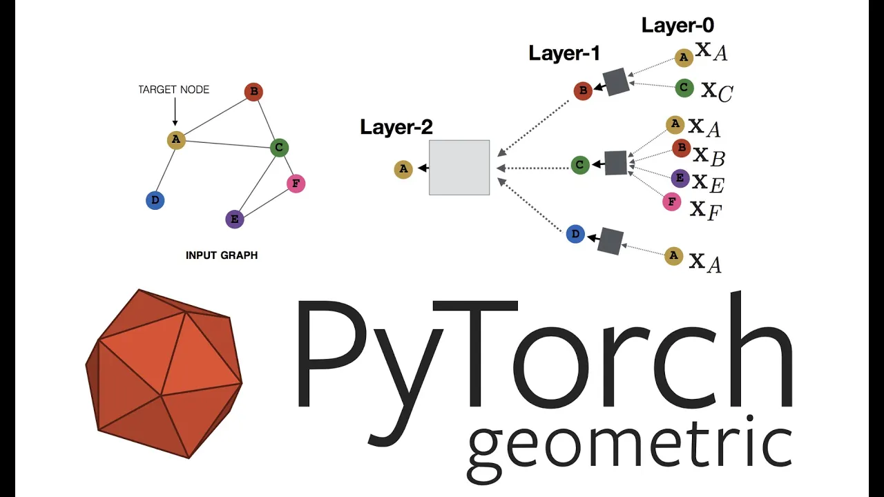
Node Classification on Knowledge Graphs with PyTorch Geometric

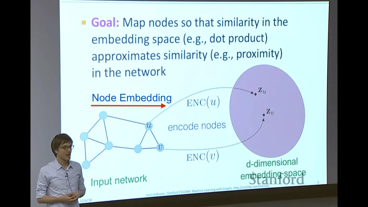
[00:00:00]hello everyone in this video we will have a look at how to build a graph new network for a specific type of prediction which is node classification in the comments it was requested to do a video on how to build such a model for one large graph i will refer to this large graph as knowledge graph in the following even though the term of knowledge graphs is a bit broader i think it comes pretty close to what we will do in the following now this video is based on the concepts of the video series on gnns i recently uploaded and therefore i won't go too much into detail on how the gnns work and the theory behind them but rather focus on how to build such a model for this node classification problem again i will use a google collab notebook so let's have a look at today's agenda so this is the notebook we will work with and first a little disclaimer parts of this code come from the pytorch exercises which you can find under this link so the structure of this notebook is first the installation of pytorch geometric and then a little bit about knowledge graphs and note classification after that we will have a look at the data set which is cora in our case and then we will build the graph new network and train and evaluate it finally i will also show you a way how you can visualize the node embeddings so the learned representation for each node so first let's talk about the installation we run these three commands which will install pytohd geometric for us so pytorch geometric is the deep learning or geometric deep learning library we will use in the following to build the graph new network this installation will only work for cuda version 10.1 so you have to make sure you're using this cuda version using this command so the problem we want to solve here is we have one large graph which is the knowledge graph which contains different nodes that are connected in some way and we don't have many individual graphs like molecules which we had in the previous videos so the task now is that we have unlabeled nodes in this large knowledge graph for example we don't know the class of some of the nodes and now we want to predict these unlabeled nodes using the information of the other nodes in the graph so this is the overall task we want to solve there exists different data sets in python geometric that can be used for this type of problem and one of them is for example karate network or cora and we will use cora which is a citation network so korra consists of around 3 000 scientific publications and these publications are the notes so papers or books or i don't know what exactly it is but some sort of publication and each of them has one of seven classes and these are the labels and one of them could for example be a neural network so it's a paper about neural networks or a paper about reinforcement learning and so on so it's ai based and we want to classify the papers additionally we have note features for each of the papers and these note features describe the content of the papers in our case this is a word vector of size 1433 and this is a representation of the content within this paper before we move on i thought it makes sense to visualize how the data looks like so this is just an example of the general structure of the core data set and by the way the cora data set is a benchmark data set and you will find it in many geometric deep learning papers in this example we have five publications so in the real data set it's around 3 000 which are linked unidirectionally this means we don't really know which of the two nodes cited the other one but we know that there is a relationship between these publications the colors represent the labels or the classes of the nodes for example two of the publications are about neural networks so paper two and four they are connected as one of them or both cited the other one which probably means they address a similar content paper one and three which are the purple ones are related to reinforcement learning and also connected to one of the neural network papers for example they use a specific network in their publication finally paper 5 is unrelated to paper 1 and 3 as it talks about genetic algorithms in combination with a special type of neural network described in the neural network paper 4.

[00:04:16]again this is just an example but the labels i used here are actually a subset of the labels in the core data set now let's have a look at the prediction problem let's assume we have another paper in the database which was cited by paper 5. we don't really know which publication type it is the task now is to classify the node using the publication types on the right with the knowledge in the graph intuitively this new node would very likely be another paper about genetic algorithms as it's first of all connected to paper 5 and secondly completely unrelated to paper 2 4 1 and 3 which are papers on neural networks and reinforcement learning we can use a graph new network now to perform this prediction for us besides the structural information about the graph we of course also have node features for each node in case of the cora data set this is a word vector like already mentioned and this word vector describes the content of the paper i'll show you in a second how these word vectors look like so now let's have a look at this visualization of the core data set grouped into different neighborhoods which i found on the internet there are around 2 700 publications and these are connected with around 10 000 links as you can see there are some significant groups of publications and using their knowledge in this neighborhoods we can easily predict the class of an unlabeled node in a graph for instance let's assume we have an unclassified node right here we can use a graph new network before message passing in that neighborhood and predict that the label is most likely blue here finally before we go back to the code let's have a look at how the node features of each publication look like the representation that is used is called back of words this essentially just means we count the number of occurrences of a specific word in each of the publications in case of the core data set this consists of 1400 words which are usually called the dictionary for example we can count how many times the word neural network relu reinforcement and so on occur this will then be a pretty good representation of the content within each paper additionally we apply some sort of normalization and then we end up with a no feature vector for each publication in our graph in the example i used a minute ago this would look something like this we also have this vector for the unclassified node just as i explained in the g n series after several message passing steps in the graph new network we will end up with node embeddings that contain the knowledge about the other nodes and connections in the graph eventually we can use the embedding of the unlabeled node and predict the publication type with it this is possible because the embedding tells us everything we need to know such as the content of this paper its citation network and eventually the content of the other papers in this example our predicted class is genetic algorithm so now that we are familiar with the data set and how node classification works let's implement this in pytorch geometric we can load the data set using this code so we specify the name here and additionally we apply the normalization i just talked about this normalization comes from torchgeometric.transforms it's downloading the data pre-processing it and we have the data available so now let's investigate what the data set looks like first of all we can print the length of the data set and we see we have exactly one graph next we can have a look at the note features this is the word vector or the back of words representation i just talked about and finally we have the seven classes which are neural network reinforcement learning and so on so the paper type so now we select this only graph we have and if we print it right here we get something like this so this tells us we have around 10 000 edges we have the masks which are the binary masks for the prediction and the training and the validation and we have finally the note features here which are these back of word representations for each of the notes so we have 2708 notes finally as we have a note level prediction problem we have exactly 2708 labels so for each of the notes we have a category which is one of the seven classes we have here so before we move on i want to show you how these binary masks look like i already showed this slide in the gene n series and this is just a quick reminder how to deal with note level prediction problems here you typically have some unlabeled notes for which you want to perform the predictions in our case we have the publications with an unknown document type this means we don't have labels for the training available for these nodes therefore they need to be masked out during the training and masked in during the prediction this can be done using the masked vectors in pytorch geometric which are binary or actually boolean vectors so either true or false next we can investigate the available number of training nodes using this train mask and summarizing over the entries so as already said this is boolean so either 0 or 1 we can see that we have exactly 140 nodes available this is a relatively small set as it's only 5 of all nodes and more specifically we have exactly 20 nodes per class the rest is unlabeled next we can investigate how the node features look like so the node features are these word vectors which are normalized and for example here we can see how the entries are normalized and this example are the first 50 entries of the first node so node number zero which is at position zero here has 1433 and the first 50 of these look like this so we have a word occurrence here at whatever word this is and these are zero because the document doesn't include these words and this is how the general structure of these note features looks like so you might ask yourself now why do we even need the graphene network can we not simply use this input to predict the class and apparently it's much better to use a graphene network it was tried out with simple mlp models and apparently the citation information is crucial to perform a good classification so the labels are numerically converted and that's why we have them from zero to six for example the label vector looks something like this next an example for the binary masks so here we have a test mask so these nodes will not be included and these nodes will be included so next here we see the edge information we can see that node 0 is connected to node 633 and so on so we have tuples of connections and this is basically our adjacency information so now that the data set is clear we can move on to build our graph newer network to do so we will simply build a simple pi torch model but the only difference is that we use the gcn layer here this is the graph convolutional layer which will perform the message passing in the first step we initialize our layers in this case we use two times the gcn layer so we have two message passing steps and then a linear output layer that outputs probabilities for our seven classes so basically if it's 100 sure that it's class number three we will have at position three a value of one in the next step we define the forward function here we pass our input which is the node feature or the note embedding as well as the edge information to our two convolutional layers so graph convolutional layers in the first one we simply pass this information apply an activation function and additionally apply dropouts these dropouts will only be applied during the training so we don't lose information when performing predictions in the second step we will use the other convolutional layer again pass our information apply an activation function and apply dropouts with a 50 dropping probability and then we have our final output layer here we apply soft max this will generate probabilities so basically squeeze our values between zero and one and the summation of all our outputs will equal to one so this ensures that we have probabilities now let's print our model so we start with the word vectors and in the first convolutional step they are transformed to the node embedding size which is 16 here we pass it here and then we have another message passing step and as you can see the output are the seven probability values that's it already regarding our new network architecture so again we use two message passing steps so two graph new network layers and then we apply the soft max to the output so we have a classification probability for each class okay now we can train and evaluate our gnn so first we build it again using a hidden channel size of 16 and then we can use the gpu if you want so we will use the first cuda device and we will put our model and the data to the device so to the gpu then we specify our optimizer which is atom and we pass in an initial learning rate and the learning rate decay here and also the model parameters as loss function we will use the cross entropy loss this is commonly used for classification problems as you know we output 7 probability values and this loss function will make sure that we will arrive at the perfect probability a probability of one for the right class then we can train the model using the strain function here another interesting part is we pass all data because each of our nodes has a note embedding or note feature vector but when calculating the loss we apply our train mask here and the same way in the test function we apply the test mask because we only want to use the nodes for which we have labels available so that's why we select only the labels and the data that is valid within the strain mask and that's it already so we can start training now i will print the loss here and you can see it's decreasing we can actually also visualize this like i did in the previous video so you can see the loss is decreasing and we can using the test function also check the accuracy so it's not perfectly high but for this example we have around 75 percent so three-fourths of the data are predicted correctly this is an example of how the output of the model looks like so for each of the nodes we get a prediction like this and here in this example we have around 95 percent prediction that it's class 2 and only a very small prediction that it's class 3 and for the others it's basically zero and this is how the output of our model looks like and eventually we will use the class with the highest probability and this is then our predicted class so here for example it's two and as you can see if we print the size of this of this output tensor so here you can see these are the predictions then we can see that we have these seven probability values for each of the nodes and remember we have only one graph object so this means we get predictions for the whole object we input the whole knowledge graph here and get predictions for each of the nodes so that's why the output shape here is number of nodes times these seven probabilities and now in this part i will visualize the embeddings and therefore i will use t-sne i won't go into detail this is a dimensionality reduction technique so this is motivated by the exercise from pytorch geometric we will reduce the dimension of our embeddings to a dimension of two and therefore we can visualize it in a simple plot and this is done in this code i won't go too much into detail on how it works but first we reset the parameters of our trained model and here i train the model again and every 50 epochs i generate a snapshot that shows how the embeddings of our 2708 notes look like additionally i will color the points in their specific class so all notes with the same class will have the same color in this plot so i built a gif out of these visualizations using the library movie pie and then this gif is saved with a frame rate of one so we have one image per second and i can display the image now using this command and as you see in the first plot everything is spread all over the place so our embeddings are completely spread but over the time so over the epochs our gnn improves the embeddings and we can see that there are some clusters so basically classes with the same embeddings appear in the same area and this is actually what the goal is to have a perfect clustering here which will eventually for new data points easily allow us to predict their class okay and again we can further play around with this model you can apply cross validation or you should actually and you can also play around with the hyper parameters like the number of layers the hidden dimension size and so on and of course you can also try out different layers another interesting example would be to include the edge features i have left a link here there's a paper on how to exploit edge features and actually they also use the cora data set somewhere down here here it is and they actually achieve an accuracy of 88.8 so that's pretty good and actually the best performance you can currently achieve with the core data set is around 90 and on this website papers with code you can actually check the benchmark in july this year there was the best submission which is around 90 and if you move down here you can see it's this ssp model and it actually also works with graph newer networks so make sure to check this out and that's it for the video today i hope this was helpful for you and if you have further questions just let me know and see you in a future video