

![#4 Machine Learning Specialization [Course 1, Week 1, Lesson 2]](https://i.ytimg.com/vi/sca5rQ9x1cA/maxresdefault.jpg)



![Logistic Regression, Sigmoid function, One vs All classification, Machine Learning Lec 7/30 [Urdu]](https://i.ytimg.com/vi/odiFMDhn3yo/maxresdefault.jpg)









![[MIS7397 Predictive Analytics] Lecture Video 10 - Model eval & dec weights | Bauer@UH BZAN PythonBA](https://i.ytimg.com/vi/vyBeUXLaY6E/maxresdefault.jpg)


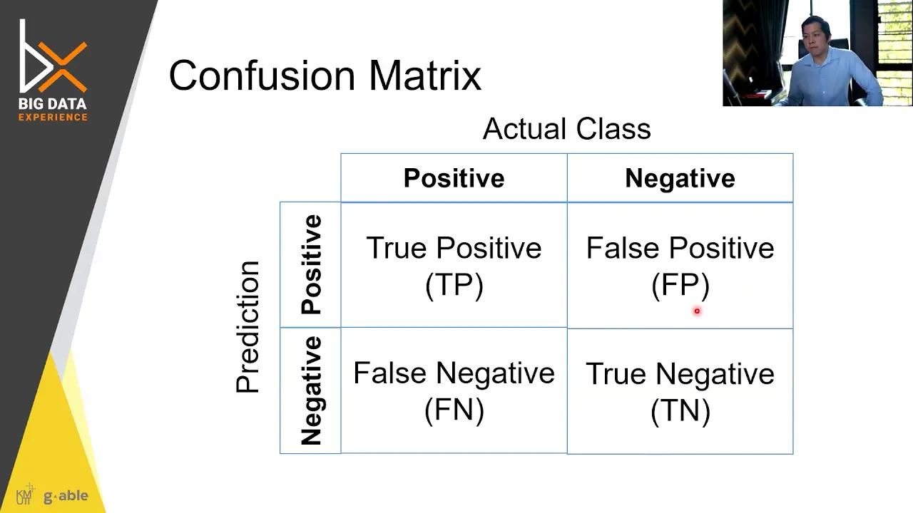
This lecture covers essential performance metrics for evaluating machine learning classifiers beyond simple accuracy, including the confusion matrix (which breaks down true positives, false positives, false negatives, and true negatives), precision (accuracy of positive predictions), recall (sensitivity or true positive rate), and the F1 score (harmonic mean of precision and recall). The lecture explains the precision-recall trade-off, showing how adjusting decision thresholds affects these metrics, and introduces the ROC curve (plotting true positive rate against false positive rate) along with the AUC metric (area under the ROC curve) for comparing classifier performance, demonstrated through comparison between SGD and Random Forest classifiers.
Machine Learning Evaluation: Performance Metrics Explained
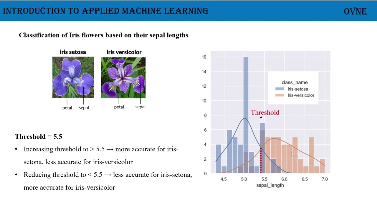
Added:what is up you guys so welcome to the third lecture of this series entitled machine learning with tensor flow and scikit-learn and this one will be talking about performance measures that is we're going to be dealing with a bunch of metrics or curves that have to do with the performance of a certain classifier or model in the previous lecture we introduced the cross-validation and how to perform cross validation on scikit-learn and this one will take a step further and introduce more interesting and informative metrics such as the confusion matrix the precision and recall parameters and by the way recall is also referred to as sensitivity as well we'll also be talking about precision recall trade-off and precision recall trade-off curve along with many of its interpretations and last but not least we'll be dealing with the ROC curve that stands for the receiver operating characteristic curve we'll see how to analyze that curve and talk about related parameter that is the AUC metric which also stands for the area under the curve metric we'll be comparing the performance of the SGD classifier that we have versus the random forest classifier in terms of ROC curve we'll be seeing how to assess the goodness of a certain model and compare performances between two different classifiers so without further ado let's get started now before you get too excited with those numbers that is 98% accuracy and stuff let's compare it to some naive classifier that is so done that it classifies all the time that I don't have a six whether there's a six or there is no sex I just predict nose so for that let me import the base estimator for that I'll create a class solid Dom classifier which overrides space estimator and just predicts a zero or return zero no matter what the data point is that is I'll return a false learn and there you go let me instantiate don't classifier as such and run the cross-validation using the stunt class passing the training data on number six over here as you can see it's yelling at me it's telling me that the score should be specified now unlike before which by default is accuracy here I have to specify it because I'm using the base estimator for that I'll specify accuracy and there you go so this dumb classifier actually did a good job ninety percent of the time is doing stuff correct not because it's doing something good but because only about ten percent of the images are sixes and a way to see this is just some the number of sixes in my training set so out of the 60,000 only nine percent or ten percent are six so that's why it's doing a good job now if I were to say classify everyone as six I'll get a bad performance right that said accuracy is generally not a preferred measure for classifiers especially when you're dealing with skewed data sets our skewed data sets are when some classes are much more frequent than others now in multi-level classification this might be more important but in this case it's not because the number of sixes is ten percent of the time whereas the number of not six forms ninety percent of the data so we say that the data set is skewed so a much better performance over here would be the so called confusion matrix so a way around this problem is to look at the so called confusion matrix the idea here is to count the number of times instances of class a are classified as Class B for instance to know the number of the classifier confused the images of six with let's say three you'd want to look in the sixth row and third column of the confusion matrix now to compute the confusion matrix you need to have a set of predictions so they can be compared to the actual targets you can make predictions on the test set but remember that you want to use the test set only at the very end of your project instead you can use the cross valve predict function so we imported it here and now let's use it so let's train on the predicted values using that particular function we pass it the classifier called by X train and the Y train six now we're ready to get the confusion matrix using the confusion matrix function so we just pass it as such the training on number six and predicted training us so we run and we can see that each row when the confusion matrix represents an actual class while each column represents a predicted class so the first row of this matrix considers none six images to the negative classes that is fifty two thousand seven hundred and sixty four of them were correctly classified as none sixes okay those are actually referred to as true negatives okay so the number of times I said no this isn't a sex is that much thus a true negative now on the other hand the remaining 1318 were wrongly classified as sixes in fact they're not sixes but this model predicted that they are sixes we call those false positives okay now reading the second row we can see that four hundred and nineteen were wrongly classified as non sixes so we refer to those as false negatives okay and last but not least the remaining five thousand 499 were correctly classified as true positives that is they are actually six and model predicted that they are indeed six so a perfect classifier would have only true positives and true negatives this is the extreme case so that said the confusion matrix for a perfect classifier would be a diagonal matrix right the off diagonals would be zero that is there is no false quantities so how can we see this well all you have to do is just fictitiously say that we've got a perfect training that the training set is actually the one trained on those six is right as such then we call the confusion matrix passing in the white train six and the perfect training as such now as you can see we don't have false wanted ease now the confusion matrix gives you a lot of information but sometimes you may prefer a more concise metric that is you want to buckle up all the information you have in just one metric now an interesting one to look at is the accuracy of the positive predictions that is usually called the precision of the classifier so that is given by the following equation where T P stands for true positives and FB stands for false positives okay so the way you can you know instead of you having to write code to count the number of true positives or just extract them from the matrix right you can just you know use the precision score so the precision score as we did in the confusion matrix we pass it the Y train sets and the white train predicted in the same order and there you go it's zero point eighty sixty-six etc now to make sure that this is correct all we have to do is just use these values over here so though plugging in the true positive and the false positive we get this quantity that is this that is five thousand four hundred ninety nine over six thousand eight hundred and seventeen which is finally zero point eighty sixty six okay now what would be the precision when we train using the perfect training data set were we fictitiously said that why training on six is the perfect training we'd get a 1 because the off-diagonals there is no false the off diagonals are zero there's no false positives or negatives so pass the white train six and the y maen perfect to get a precision of one right now there's another metric that is used and it's called the recall so the recall is defined as the number of true positives over true positives plus false negatives now this has other names such as sensitivity or the true positive rate TPR okay and find those in different references now this is actually the ratio of positive instances that are correctly detected by the classifier and a way to you know use SK learn library is to import the recall score function and in the same way you could pass the training sets and your recall score would be 0.92 91 now let's see if this is correct go up here you see that the number of true positives is as before five thousand four hundred ninety nine and the number of false negatives is four hundred and nineteen so doing a bit of math at this ratio that is indeed zero point nine two nine one okay so now what we can see here from the different metrics is that your own classifier is not as good as it sounds right um using those different metrics we can see that the precision is 0.8 and recall score is 0.92 and those metrics do not report its accuracy right as the data set is skewed that is some classes in our case six are more frequent than others okay now indeed you can find many metrics many performance measures in machine learning that combined for example the recall sensitivity metric with for example the precision so there's a very known metric called the f1 score that is equal to this ratio that you see over here so in our particular case this evaluates to this quantity over here that is roughly this ratio that is around 0.86 and a proper way to do this on using SK learn metrics is to import the is to use the f1 score function is to use the f1 score function so as we did previously we pass it the white train six along with the white train predict and we can see that indeed evaluates to zero point 86 now the f1 score is also referred to as the harmonic mean okay so the harmonic mean the harmonic mean of precision and recall because as you can see over here we've got a sort of mean down here it's the mean of the inverses of you know the precision with the recall right so it's as if we're taking the average of the inverse of precision and recall and then we're again inverting this metric right because if you'd look at 1 over f1 it looks like this right so it says if you're averaging 1 over precision it's 1 over with 1 over recall and then taking the universe it's sort of like resistors in parallel in terms of electrical circuits so let's say you've got two resistors they're in parallel well this is a way of doing it sort of because 1 over R equivalent is 1 over r1 plus 1 over r2 but there's no you know 1 over 2 right so yeah this is referred to as the harmonic mean and why is it so important it's because the harmonic mean gives more weights the traditional mean so if I were to take precision put + recall over 2 you know precision and recall have the same weights right as you can see over here this is a traditional mean right whereas if you take the harmonic mean you've got more weight towards lower values so let's say recall is doing way bad right whereas precision is doing a pretty good job so if recall is going to zero that guy goes to infinity right whereas 1 over precision let's say in the best case it's 1 so 2 over 1 plus infinity that would give you a zero harmonic mean whereas if you do the traditional mean you get a 1 & 0 over here you'd get 1/2 right so the harmonic mean is more of a pessimistic metric if you have one of those guys going to 0 then the harmonic mean would go to 0 whereas the average the traditional mean would not write 1 by the way in case I didn't mention it here so ya if ya if you're doing a pretty good job it means that all's positives and false negatives are zero right so in that case the higher the precision so the precision is bounded between 0 & 1 right higher the better and so as the sensitivity the higher the better right likewise the harmonic mean is also bounded between 0 & 1 but finally we can say that the f1 score favors classifiers that have similar precision and recall right so let's say the precision is 1/2 and the recall is 1/2 right let's say we've got equal precision and recall um let's say they're 1/2 we get a 2 over 2 plus 2 that's a 4 so we get 1/2 in that case it would be harmonic mean would be equal to the precision and recall right likewise if you choose any other you know the precision is equal to recall then say they're equal to X then what you get is this ratio that is finally X so in case precision is equal to recall then the f1 score is also equal to both parameters right X so as I said f1 score favors classifiers that have similar precision and recall this is not always what you want and this is not always good right because in some contexts you mostly care about precision and in other contexts you might want to take a look at the recall right for example if you're trained a classifier to detect videos that are safe for kids right on YouTube for example say the YouTube team is implementing it a classifier that wants to detect videos that are safe for kids you'd probably want to prefer a classifier that rejects many good videos but keeps only the safe one so if you're rejecting many good videos you'd have a low recall but if you keep safe ones you'd have a high precision rather than classifier that you know has a much higher recall but that's a few really bad videos show up in your product on such cases you might want human interference right so that they could check on the classifiers a video selection now on the other hand suppose you train a classifier to detect but say shoplifters on surveillance images in that case it is probably fine if your classifier has only let's say forty percent precision as long as it's recall happens ninety-nine percent of the time now the downside here is that you can't have it both ways increasing precision would reduce the recall and vice-versa okay the higher the precision is the lower is recalled cannot boost both parameters at the same time right and thus you have the so-called precision recall trade-off okay so the higher one goes the other is pushed down and vice-versa okay so to fully understand this trade-off let's first take a look at the stochastic gradient descent classifier right the SGD classifier and it's really worth looking at how SGD makes its classification decision right so for instance it computes a score based on a decision function and if the score is greater than a certain threshold it assigns the instance of the positive class or else it assigns it to a negative class so the way you can understand the decision function is let's say for example I grabbed again my SGD classifier over here and I am going to predict some certain digit I'd say this digit is I don't know let's say it's the third row of X let's see what it is so first all reshape it 28 by 28 matrix right then I plotted this number over here there's another number 0 0 so again this classifier is predicting whether a given digit is 6 or not though this is clearly not a 6 see it is not back to the 3 example there digit is also not a sicko you get the point so we're getting either a true or false let's pick a certain set me let me organize the clay here I'll get rid of this that let's control the digit digit is a index right that 19 this number and false also again also again again okay so I picked this index it gives me a 6 and it's predicted as true okay well it would be interesting to look at another metric so as you can see here we've got a hard decision output right so it's either true or false well SGD classifier comes with another soft decision function that gives us a number between minus infinity and plus infinity the higher it is the more confidence we have that given digit is a sick and the lower it is the less confident we have right oh let's pick another number let's say it's 5 we get a negative so normally the threshold is around zero but and scikit-learn does not let you change this threshold directly but does give you access to this number right you have it here then you could go ahead and set a threshold rule right so you could vary your threshold you should be careful here once varying the threshold you're you're also changing your precision and recall so the threshold here let's say the output is referred to as the Y score right and in case the Y score is greater than some certain threshold and we'll set the threshold let's say to zero zero and there you go you get the same prediction as the predict function right let us change it back to 6 true true right whereas if you set the threshold to high let's say 200,000 you had a false right so if you set it too high you're actually increasing your precision but you're decreasing your sensitivity or recall and vice versa if you're putting this threshold too low then you decrease the precision and increase the recall right so if I were to draw what's going on over here say we're predicting 6 all the time so let's say this is the score or and this is your over here you've got some given inputs to predict let's say this is a six is a six this is another and put it here and then once it starts decreasing so this is the zero start mixing so it might mix it with a 5 or a 1 then I'd get a 6 again for some noisy reason boo and seven maybe and nine and a 1 so the less it is the more sure we are it's not a six it doesn't look like it's the chances are the core is really negative right you're not going to see any sickly you might come on I don't know set a threshold here here right or even I don't know here even here and so on so if you're going to set a threshold and take a look at the precision precision actually increases with threshold though once you set this threshold to high right call this t1 for threshold 1 t2 brush hole to and t3 threshold 3 so once this threshold is too high your precision actually increases of course I mean you're setting a very high threshold so that you predict a 6 as you can see at t3 you do no mistake because the precision is 100% right now as precision decreases you can see here I've got you know how many times do I have a 6 I have a 4 out of 6 times so 1 2 3 4 5 6 4 out of 6 that's a 66% right vision and over here 1 2 3 4 when I set the threshold to t1 I predict 1 2 3 4 5 right 5 out of 9 so that's around 55% right so as you can see here the higher the threshold the higher the precision but the higher the threshold the lower the recall okay so if I were to compute the recall over here you can see that according to the formula over here true positive over true positive plus false negative I have to count the number of correctly identified time so that's a 3 over 3 plus how many times I didn't identify 6 when it was actually at 6 thus a false negative we've got a 6 over here 6 over here we have any other sixes no - we got a 3 over 5 over here that's a 60% right let's do the same thing here so we identified four sixes right here and we've mistaken one six oh that's a four out of five is 80% right now once you go here you identified all the sixes so all the sixes are regardless of the number of times you've mistaken none six to be judged as a six for example the seven to write recall doesn't really care about that recall just cares about how many times you mistake in a six to be something else so that said we've got one two three four five five sixes and there's no misclassified six so that's a five out of five which is a hundred the idea here is that the hardest threshold the less sensitive you are the let's recall you have but the more precision you will achieve right there's this trade-off that we're actually talking about actually let's do something even more interesting let's actually plot as a function of threshold how the precision and recall behaves so it's quite good to look at those curves so precision and recall versus the decision threshold to go back down here first from the metrics let's import the precision recall curve right from that and actually use this function using your brain values six strain values and some scores now we need the scores right and the scores you can actually use the cross valve product by passing the classifier ad classifier along with the training set and the reigning 6a training the number six set you can pass the method over here there the decision function so that we get this course right wait a bit there you go so if you take a look at the scores there you have this array of just real numbers okay so from the precision recall curve we can actually get the Precision's though recalls right and the thresholds there you go that's the precision that's the recall and here's varying thresholds so this is a really handy function and yeah you can you can get what we're actually talking about now now to plot all I have to do is just you know thought as we said recisions versus threshold bought it in blue and label it as is there's an error over here Oh different diamonds is that take a look at vision oh there's a difference in one eye because it met one there you go okay yeah I don't like the dotted one let's stay with this that's on top of that but the recalls in a hand Mabel the axes a slave of the x-axis as vision threshold the y-axis has values and let's place a legend that's right and as you can see there's a lift over here so actually let's bound the Y limits between zero and one so that the figure looks but okay you go better voila Oh again as we were saying here with the threshold the higher the threshold is precision increases recall decreases how according to this in this particular data set now using this curve you can easily select the threshold value that gives you the best precision recall trade-off or your task and another way to express this in case you don't like to see a plot with two kurzon in case you want to see only one plot well you can do this you can actually plot precision versus recall how do you do that well open another plot this plot precision versus recall as such a given X label all recall and a y label all okay let's limit the x and y axis between zero and one cuz those values are between 0 & 1 so axes on wine there you go oh yeah and as you can see over here like after 90% of recall the precision starts falling rapidly look at this drop over here it was falling linearly as you can see before a 90 percent recall for you and after that it just you know shoots down right that said you will probably want to select a precision recall trade-off just before this so right over here for example around I don't know around 80% recall you can just say I want to operate in this region right go an 80% recall and a 90% it's almost 90 percent precision but again this choice depends really on the context on the application you're working with for example and other applications that say you're you're training a certain rocket and you don't want the rocket to do any you know you're shooting up a certain and a war battlefield right and you don't want this rocket you know to you know have any false alarm right you want a very high precision right so in that case no your priority would possibly be to focus on precision for any recall so you want as - precision as possible so it's really application dependent so back here again let's suppose you decide on a 80% precision you look up the first plot and you find that you need to use a threshold of about I don't know figure out or going back here how much is an 80% recall so 80% recall we can take a look at the recalls here starting from 0 up to 100 we want the first value that you know cuts 0.8 a true - - I want the first I say false value or the last true value how can I do that the way to do that is well we can write a lambda expression i for i X and enumerate so we're going to pass element by element in this true false array and this boolean array and set the threshold to 0.8 if X okay let's take a look at t there you go this is the list so I'm interested in the last element right there you go this is the first element over which the recalls is greater than 0.8 so to make sure I'll just pass it as such or as such so it's zero point eight zero zero one right um let me stick with this and that's what happens when we just trespass it it's less than 0.8 okay so there you go zero point and let's save this index index let's say operating index okay this is your recall let's take a look at the precision for this particular index it's 0.94 so right here 0.8 0.9 for let's say we stick with that right so that's also so this is my recall operating recall this is my operating precision what about my operator and threshold is so zero of course not if you look at it it's that much thirty eight thousand eight hundred and thirty nine right so though that's your operating point and so you decide to go and get your training values in this region so why train predict operating let's actually call it it as an 80 percent recall right so get your scores and choose the operating threshold right there you go so this is a true/false array and let's actually check for this particular array what is the recall and precision they should be if I go ahead and print them it should be that much right well let's verify if that is correct how to do that well as we did previously over here we're going to use the precision score and the recall score right though let's do that decision or on white train six and why train deaf to 8000 point nine four four one exactly let's compute the recall right there you go zero point seven nine nine well pretty close to the zero point eight right okay oh we have learned this section how to get our desired precision and recall and how to operate in this region for a binary classification problem and as you can see we can create any classifier with a desired precision by just increasing or decreasing the threshold we want a high precision you just increase the threshold but bear in mind that your recall is going to decrease according to these two curves right and in many applications having a high precision is not very useful okay you can be able to classify a correct six but you're going to end up misclassifying a lot of sixes so another common tool used with binary classifiers is the so called ROC curve that stands for receiver operating characteristic it's very similar to the precision recall curve but instead of plotting precision versus recall the ROC curve plots the recall or also the true positive rate versus the false positive rate so the false positive rate is only the ratio of negative instances that are incorrectly classified as positive it is actually equal to 1 minus true negative right now the true negative rate is also you can see in references that true negative rate is also referred to as specificity hence the ROC curve plots sensitivity the recall or the true positive rate versus 1 minus specificity can such recall versus its sensitivity vs 1 minus specificity that's the ROC right so the way you can do this is using the ROC curve function from SK learn you get the false positive rate and the true positive rate along with the decision thresholds you call the ROC curve function on the training said that you have and the scores there you go so let's plot it as we said it is true positive rate or recalled versus the false positive rate or 1 minus specificity right there you go give it a X label of f PR or false positive rate the Y label be PR or true positive rate also the recall over here I'll put between brackets 1 minus specificity now a region of you know comparison would turn out to be the y equal x function right though on top of that I'm going to join points 0 0 1 1 as set right and I'll specify the axis values are only between 0 & 1 the X and the y there you go let me the linewidth over here cuz it barely shows right there you go okay so again over here as with the case of recalled precision you've got a trade off here so the higher the recall is we're here more false positives classifier produces this y equal x line or dotted line represents the ROC curve of a purely random classifier so if i just build like the dumb classifier a classifier that just classifies randomly this is what you'll get the y equal x line over here so a good classifier stays as far as possible from this dotted line and of course up towards the top left corner right it's not going to go down over here and that it's really bad in that case a random classifier would have done better than a ROC curve that is below right so one way to compare classifiers is to measure the area under the curve also referred to as AUC right a perfect classifier will have on AUC equal to one that is if this classifier is in the perfect case which is not attainable but well it depends on the training data and the testing data but let's say in the perfect case you have a line over here like joining this point to this point and this point to this point well in that case the area under that curve would be just you know square the axis it's a square so side squares 1 square that's the one so in the perfect case you have an AUC equal to 1 right whereas in a purely random classifier the dotted line you got an a you C equal to 1/2 it's the area of the triangle base times height over 2 that's 1/2 or 1/2 the square right that's 1/2 instead of you having to go you know and compute this area numerical functions or I don't know what you got a function there and the SK learn metrics for you so all you have to do is import ROC on the score AUC underscore score such and using that particular function you pass your training data and the scores in our particular case we've got a not so bad actually we've got a really good AUC 0.99 so let's do something with this metric let's actually train using a random forest classifier we didn't talk about random forests but let's use this just for the base of fairies before random forests I'm going to you know from SK learn the tricks I'm going to import the random Boris pacifier oh stop metrics it's ensemble there's a classifier it's not a metric you know how sometimes when you're coding it's been a long time you're coding you just you know in few stuff but that's okay so using this forest classifier going to call an instance of random forest classifier as such and we're going to call the cross the deck that we will pass the forest classifier along with the training data the training six data set the method to predict Robo give it some time to compile and the reason the method is called predict proba is because it outputs probabilities this might take a while don't worry that it executes okay so there you go take a look at probabilities there you have it and actually plot the ROC curves we don't need the probabilities we need the scores and the scores are actually the second column of probabilities right so bigger or scores as such and we'll call the ROC curve why train six so the rock will pass it by train six and the forest boards right we're going to get both positive rate of forests along with through positive rate of the forest classifier and the thresholds of for it's right there you go so now let's plot a rockers of the forest and SGD classifier that we have on the same plot to do this all you have to do is actually go let's let's get the code from here and just add one line of code right the line of code we want is f PR underscore forest and TPR in this core for civil label so label per here all it SGD and I'm going to plot it dotted red okay that's the SGD here mister forest and to plot the legend but an error there you go as you can see as GD over here whereas forest is way up so random forest is doing better convince yourself just compute the AUC score of the forest so zero point nine nine nine whereas for the SGD is zero point nine nine one inch site so as you can see what I'm trying to say is that the higher this guy is the more squeezed it is up to the top corner left right - yeah this is it thanks for watching if you enjoyed this lecture please consider subscribing to my channel liking this video sharing it on social media and if you have any questions whatsoever just leave a comment down in the comment section below I'll make sure I'll get to it as soon as possible
Up Next

Open Systems: TEK, AI & Embodied Cognition | MIT Symposium
@ArtsatMIT
416 views•2021-05-12

Secure Multiparty Computation (MPC): Foundations & Challenges
@SimonsInstitute
7.3K views•2015-05-28

Bypassing Tor Censorship: Bridges and Pluggable Transport Guide
@Coding_ForEveryone
397 views•2024-06-11

Neural Networks Explained: Math, Layers, and Learning Fundamentals
@3blue1brown
21.9M views•2017-10-05
Related Study Plans & Knowledge Roadmaps
Structured learning paths in Artificial Intelligence