












![FastNeRF: High-Fidelity Neural Rendering at 200FPS [Extended]](https://i.ytimg.com/vi/mi5b142WEmw/maxresdefault.jpg)

![3D Gaussian Splatting [Paper Review]](https://i.ytimg.com/vi/xTp88ZOtm58/maxresdefault.jpg)


![[EUROGRAPHICS 2022, STAR] Advances in Neural Rendering](https://i.ytimg.com/vi_webp/ul9hFFtWYv8/maxresdefault.webp)

Neural Radiance Fields (NeRF) represent scenes as continuous volumetric functions encoded by neural networks that take 5D coordinates (3D spatial location + 2D viewing direction) as input and output volumetric density and RGB radiance values, enabling state-of-the-art view synthesis by combining coordinate-based neural representations with classic volumetric rendering techniques; the key innovation involves using Fourier feature mapping to transform input coordinates into higher-dimensional spaces, which enables neural networks to learn high-frequency functions necessary for capturing fine geometric details and view-dependent effects like specular highlights.
Neural Radiance Fields for View Synthesis | Matthew Tancik
Added:Fundamental concepts of 3D computer graphics, specifically ray tracing, volume rendering, and camera projection models.
Core deep learning architectures, particularly Multi-Layer Perceptrons (MLPs) and how they represent continuous functions.
Coordinate systems and spatial transformations, including how to manipulate 3D rotation and translation matrices.
Basic signal processing concepts, specifically the spectral bias of neural networks and the role of high-frequency positional encodings.
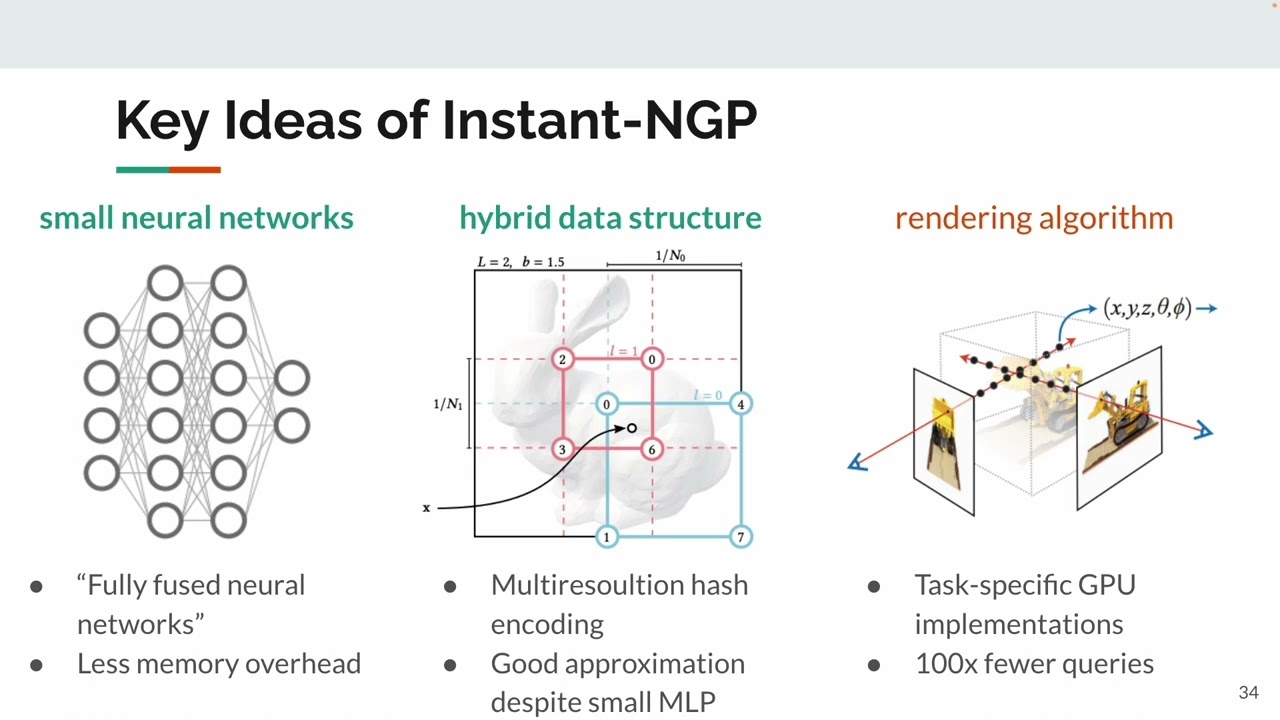
Accelerated neural rendering methods, such as Instant NGP (Neural Graphics Primitives) and sparse voxel grids, to resolve NeRF's computational bottlenecks.
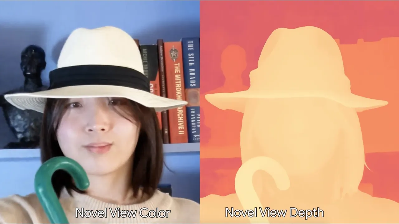
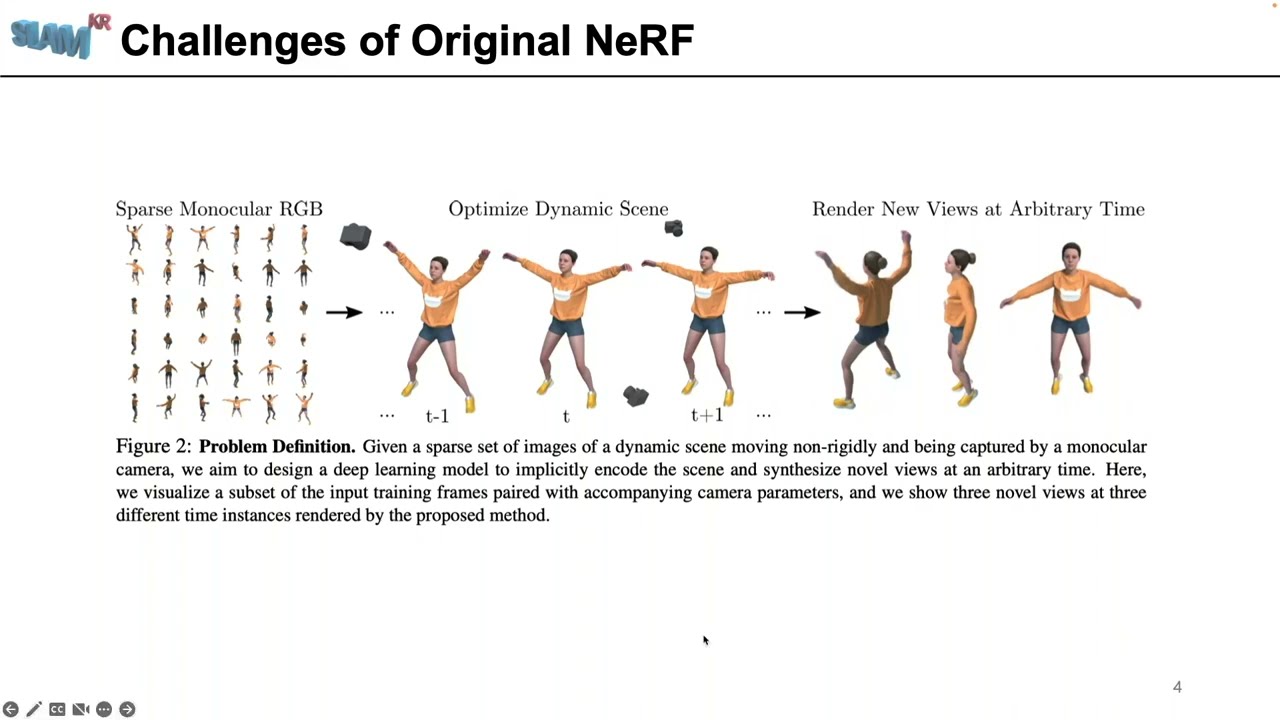
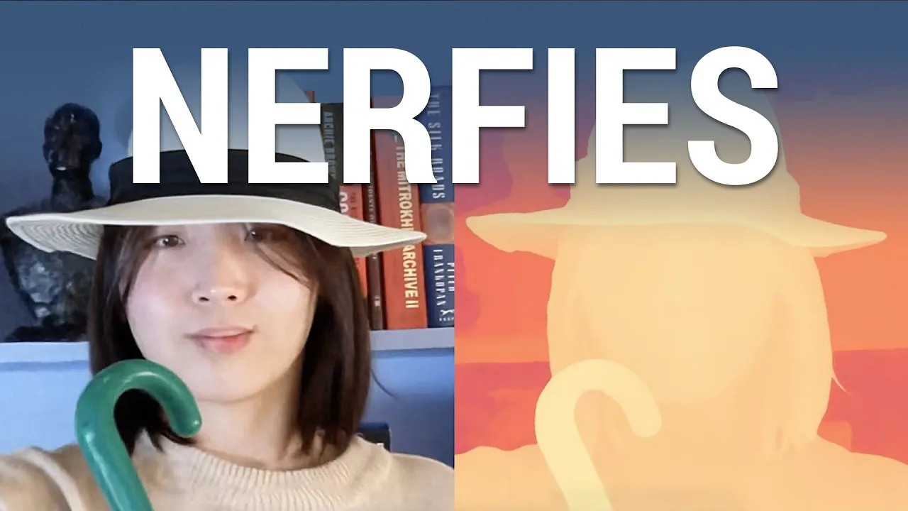
Dynamic and deformable NeRF variations (e.g., D-NeRF, Nerfies) that reconstruct moving objects and temporal sequences.
3D Gaussian Splatting as an alternative state-of-the-art representation for real-time, high-fidelity view synthesis.
Generative 3D modeling pipelines, including text-to-3D synthesis models like DreamFusion that leverage NeRF architectures.
Large-scale scene reconstruction frameworks, such as Block-NeRF, used for mapping urban environments from diverse camera angles.
31.7K views648likes49:10Original Release: 2020-06-29
let's get started so today we're happy to have Matthew 10 chick here he is a PhD student at UC Berkeley and he did his master's at MIT has worked a lot on computational photography computer graphics computer vision and very recently on a few sentences he has developed at his core first the neuro radial gradient field approach that most of us are familiar with and very recently the morphia reticle insights into the few features for all kinds of applications so I'm very much looking forward to your talk Matt thanks for coming thank you thanks for the intro so I'm Matt I'm a second year PhD student at Berkeley and my advisor is Rin hyung and I want to thank you all for giving me this chance to give this talk today I've always been a big fan of a lot of the work that you guys do now feel free to ask questions as I go there'll be time at the end as mentioned for additional questions so in this talk I want to go over two projects the first is nerf which is a view synthesis method that uses no radiance fields and then the second is the follow-up work that investigates some of the observations in nerf this is joint work with a number of collaborators most of us are from Berkeley with the exception of John Baron from Google and Robbie Robin war thief from UCSD I want to quickly highlight bin Mildenhall and Patrol Srinivasan who both contributed significantly to both of these works so first I'll talk about nerf which is representing scenes as neural radiance fields for view synthesis there's been a lot of recent progress in using deep learning for novel view synthesis we're able to produce pretty incredible photorealistic content from sparsely sampled imagery for this talk to focus on the specific problem of view interpolation this is where you get multiple input views of a given real-world scene along with the corresponding camera poses and then you use them to render photorealistic new views of that same scene that interpolate between the given views this is where the remote presentation may start to break down a little bit so on the left you should see jerkiness between with like large pixel shifts between the inputs and then hopefully on the right the video looks smooth this video includes the interpolated views that are being synthesized if the right video does not look smooth you'll just have to take my word for it and also all these videos are posted online so now that we have this problem statement how do we solve it so at a high level an approach that has been very successful so far is to essentially take your set of images and then use them to predict a 3d discrete volume representation such as a voxel grid you can then render new views by compositing along the Rays a lot of the recent successful methods can be roughly described in this way so this includes methods like soft 3d which were state of the art prior to deep learning and they use traditional stereo methods to estimate an RGB alpha volume recent work in multi plane images or MP eyes can also be thought of in this way since they're essentially a estimate of a particular frustum shaped layer RGB alpha representation that uses classic alpha composition along the Rays in order to render new views other cool works like neural volumes use the strategy to learn these like cool little dynamic 3d videos so this successful strategy for photo realistic view synthesis combines machine learning with with traditional RGB alpha volume rendering models these discrete grid based representations are really easy to integrate into 3d CNN pipelines since you can unprojected grid and then we run a 3d CNN to predict the RGB Alpha voxel grid the alpha composition operation used for rendering is trivially differentiable and it plays nicely with gradient based optimization so the 3d CNN networks can just be trained on how well they render out the held out views this is great for optimization but you start to get a really bad scaling property as the resolution increases this gets even worse for some of the state-of-the-art algorithms which use multiple 3d grids to represent the larger scale scene and it's not uncommon for these to use multiple gigabytes just to represent a single scene now thanks in part to you all there's a totally different approach for representing 3d content that's been gaining a lot of traction in this case we have a neural network that represents the shape by encoding a continuous function in 3-dimensional space here we have a visualisation of one version of that idea where the underlying function is a continuous occupancy field so the function should be zero for all points outside of the object like this binge in this case and then the value 1 for all points inside now by supervising it with ground truth occupancy you end up with a shape representation that is the network itself representing shapes as occupancy is just one option you can do other underlying continuous functions like sine distance fields like in deep SDF however they all share this common attribute that the shape itself is restricted to be on a surface which exists as a level set of the network so in order to extract and render the 3d object you essentially have to find a bunch of zero crossings in the network itself so most of these methods supervised with ground truth 3d information which isn't quite usable for view synthesis however more recently there have been methods that use networks with images as input but they have to differentiate through an iterative zero crossing solver in order to figure out where the surface is located for each ray so far this process is easy to defer it's not as easy to differentiate as volume rendering and this arises from the fact that they have to represent the shape as a surface of instead of a volume but the compression benefit is huge you can save as you can see the like between ten to a thousand times more efficient compared to a volume based representation and this is great because these these voxel grid representations are too big and that's really a bottleneck for those methods so in this project our core idea was to combine the benefits of both these methods so we use a neural network instead of a voxel grid to encode a volumetric representation of the scene and then when we want to render new views we use the same volume rendering style that has achieved these great results in the past so these are the key details I want to cover in this talk for Nerf and I'll expand each in turn so starting with the first one let's take a look at how we represent the scene as a fully connected neural network so we can replicate represent any arbitrary scene as this network which in this case is just 9 layers and 256 channels so I think this ends up being around 5 megabytes so it's a pretty small network the network then takes in a continuous 5 D coordinate containing the 3d location X Y Z along with the 2d viewing angle theta Fe and then outputs the volume density Sigma which can be thought of as the opacity at that location as well as the RGB value representing the radiance emitted from a particle at that input location along the viewing direction so in contrast to previous work with volume representations here we're just vid fitting a continuous function approximator to the volume without Everest and shading a grid of individual samples this is a pretty big deal because it allows us to trivially add more dimensions without incurring any extra storage cost if we wanted to do that with these traditional representations adding those extra dimensions would be prohibitively expensive but a nerve we can do this almost for free by just appending a few extra numbers to our input to our network and then the network can decide how to allocate the capacity to represent the important parts of the function so let's take a look at how the rendering model is used to synthesize new views from this representation to render each image from the scene we need to estimate how much light of each color makes it out of the volume along each camera ray so here's a visualization where we have two images of this lego bulldozer and to render each of these views we query the network at a bunch of discrete points along the path for you train these are then fed through a network and the output let the corresponding colors and volume densities are output which are then composited along the Ray to compute the single color so we can take a closer look at how this rendering works so to compute the color for any camera ray that passes through the volume we need to estimate the 1d line integral along that Ray and we do this with a pretty simple approach where we just query the MLP at a bunch of samples like this and then we use a quadrature estimate for traditional volume rendering to estimate its continuous integral so this will compute the color C of any camera ray as the sum of contributions from each segment of the Ray through the volume and each segments contribution is the segments colors C sub I weighted by an estimate of the transmission T sub I this computes how much light is blocked before reaching that segment and finally it's also multiplied by this alpha which is the amount of light emitted by the segment and this is a function of the segments length delta T sub I and its estimated volume density Sigma this is essentially the same as the opacity of the segment so at first glance this parameterization may look different than standard alpha compositing that you may be used to but they're actually pretty similar in practice and this is essentially a continuous analog of alpha compositing so most of the previous methods for view synthesis use discrete volumes as a volume rendering model where the opacity is directly parametrized as alpha this implies that there's a constant step size but that doesn't really matter since in the cases they're interested in the output voxel grades have a fixed resolution anyways but in our case we specifically changed the output scalar to Sigma which is often referred to as an extinction coefficient or differential volume density at each point in space and then using Sigma instead of the standard alpha is crucial because in our continuous representation it allows us to render images where the distance between these points is no longer fixed like they are in a standard voxel grid so despite the fact that we learn a continuous representation of the scene the resolution of our model is still limited by two main factors the first is just the resolution of the input images which we really can't do anything about unless you get a better camera and then the second is limited by how finely we sample the points along the Ray now if we dig into that a little bit deeper you can imagine that the best solution would be to sample very densely however this can be really slow because this basically requires passing each sample through the network so to make this a little bit more efficient we do a two pass hierarchical volume rendering which increases our effective learn'd resolution given a fixed sampling budget so in the first round we just sample regularly in in regularly simple sampled like linear points along the Ray and then we can calculate the accumulated color using the equation that I previously described and if you remember the accumulated color is just a weighted sum of each segment colors so if we normalize the per sample of color weights we can treat them as a probability distribution and this tells us roughly about how much each location contributed to the final color then we can compute a second set of sample points simply by drawing these additional samples from this probability distribution this means that we'll get more sampling precision around the object boundaries where the opacity goes from low to high and this is where we want the the more samples because we don't really want to do extra samples in free space nor do we want extra samples in the object itself so this strategy has a similar feel to important sampling since we're trying to approximate an integral and we're doing fewer samples by more intelligently allocating the samples to where we expect them to actually contribute to the underlying integral this isn't a perfect solution since our core samples still need to be packed tightly enough to hit the fine details however we find in practice that given a given like sampling budget this strategy seems to always outperform just one round of linear sampling so another significant difference between our model and the models more typical and view synthesis methods is that we allow the color of each of any 3d point to vary as a function of the viewing direction this is why we refer to the learned function as a radiance field as it represents a continuous field of particles in 3d space that emit light and the radiance submitted by each particle is a function of the 2d input so our representation can also be thought of as like a volumetric version of surface light fields which represent the scenes of meshes with V dependent emitted light if we manipulate the directional inputs while keeping the XYZ locations fixed we can visualize what like we can visualize what view dependent effects are encoded by the network so so here's a visualization of this idea for two different rendered synthetic models and what we're doing is we're visualizing the different view directions he given a fixed X Y Z location so in one case it's on the ship in the other case it's in the water and what we see is that as you rotate in these two cases you get the specular highlights that appear and the corresponding colors at those points also show these specular lobes so we're able to capture this view dependent effect okay so now let's take a look at how you would actually optimize one of these Nerf networks if we go back to the expression for the accumulated color along each Ray it's clear that the final computed color is trivially differentiable with respect to the color and volume density at each sample and therefore it's also differentiable with respect to the parameters of the network that outputs the colors and volume densities so this lets us optimize the network's parameters by using stochastic gradient descent just to minimize the rendering error of the network along with the input images so to put this in context suppose we have a set of input images distributed hemispheric Lee around an object like this at each training iteration we'll just choose one of those images and render the Nerf from that camera pose and then take a gradient step on the l2 loss comparing the rendered output with the ground truth training image then over the course of training the simple multi-view consistency will encourage the network to allocate volume density allocate high volume density along with accurate colors at the locations where the surfaces actually exist in the underlying scene so that was a lot of description I think it's useful to take a look at some results so these are all real-world results where the number of images varies from I think around 15 up to 60 or 70 as you can see we can capture realistic like transparencies and reflections these fine details here's another example reflections it it works for like large scenes and here's a smaller scene and it also works for 360 real world scenes may I ask a quick question so this is super impressive results I assume like this two-stage sampling is important to get like all the defined details for the like for the image synthesis like when you do the training however like in the beginning the network doesn't know the geometry right so it seems like the sampling procedure that I described will not yield useful samples maybe does it still converge even for like this this first course step samples like like non-uniform like maybe non-uniform in space yeah so so in the first the first course samples are uniformly spaced but then we randomly like shift them forward and backwards so that during training it can kind of see the whole space and what we really just require is that this uniform for a sampling that each point like hits the object at least once or is around the object because you sort of create this like you can think of the sampling rate as creating sort of a cloud around where the object actually exists and then the second stage really tightens that to the actual shape of the object so in practice I think we do for these scenes I think it was like a hundred and twenty eight samples in the first stage and then an additional hundred and twenty eight in the second and it seems like all these stages are always part of the optimization from the start there's no bootstrapping or something no that we use them both at the start all right thanks you use two networks right for the hierarchical something two different networks no we use the same network we just sample we just put in different locations for 100k then maybe okay so yeah we find that this idea outperforms prior work that has also tried to represent scenes as continuous functions that are encoded by ml piece and so here's an example in synthetic data and we can see that the scene representation networks or SR ends are unable to represent the same level of detail and their representation is also not consistent between viewpoints since they use a recurrent network to march race through the representation so we can see the same difference on real data where the Newark is able to represent these higher details on the objects we also find that it's more consistent across views compared to our groups prior work called local byte field fusion this was a blend between multiple MPI representations due to limitations in the range of views that can be rendered from each MDI and then finally we also find that we're able to represent more detailed content compared to the state-of-the-art neural volumes work that uses a single sample volume however it's limited by the discrete resolution so here are some more synthetic scene examples and for each of these we render 100 inputs input images that are used to create a Nerf to synthesize a full hemisphere of inward-facing views it's worth emphasizing that this is pretty difficult in practice because if you think about how many images you'd actually need for a full Nyquist sampling it'd be orders in orders and order some more magnitude more images so the fact that we can do this with only 100 images with these view dependent effects is we think pretty impressive here we can do a similar visualization to that ship that I was showing earlier with the view dependent effects and here what we're doing is on the Left we're just doing the standard rendered views for different camera angles and then on the right we're fixing the camera location to be fixed and then we're changing the view directions based on the camera on the left and this allows us to see the view dependent effects that the network has learned so these are like the specularity is in the TV and on the table and we can do the same for any of our scenes so here's another one of a stove and we can see the reflection on the metal of the stove is changing with the different angles we can also visualize the geometry that's represented by the Nerf by computing the expected termination depth within each volume of each ray and this essentially computes a depth map for the volume and visualizing these demonstrate that the Nerf representation from images alone is able to represent this detailed geometry we're even able to resolve really fine details like in this case which has fine occluders which are typically problematic for standard estimation algorithms and this is cool because it shows that the Newark is not just strictly useful for hue synthesis and that the underlying 3d information that's recovered is better than you might expect because the training loss forces there to be a multi-view consistency between all of the input views we can use this detailed geometry to augment scenes with virtual objects and render accurate occlusion effects so here we're just inserting a little ball and as you can see as it moves along a 3d path the occlusions are pretty convincing so even though we use a volumetric representation of the scene the Nerf seems to learn a geometry representation that corresponds to the actual surfaces and it doesn't just distribute opacity throughout the scene like a fog which happens to some other view synthesis methods and so we can kind of visualize that by trying to invert the final volume into a mesh by doing of marching cubes and we can see that we can produce pretty detailed mesh geometry so here's a little toy bulldozer so going forward I think there's a lot of interesting issues to address one of the big downsides to nerve is that the training and inference time is really slow so training for a single scene takes about half a day and then rendering a single frame takes about 30 seconds so this is mostly because when you render each frame the number of queries and network has to make is really large for I think a 1 megapixel image ends up being almost a quarter billion queries so it's almost impressive that we have architectures that can do this in 30 seconds now though it's worth noting that during inference time we have a lot better idea of where the actual content is so we can be smarter about how we allocate those samples so anecdotally we find that just limiting the queries to a course hole around the object can speed up the rendering by almost an order of magnitude however this is just a preliminary result and we think that with further investigation you could really impact the training and inference speed which would be a very useful for a model like this so another cool direction is to extend the nerve representation to enable more graphics functionality so right now we can just render a new scene new views of the scene but what we really want is to take photos and then recover full graphic assets that can be composed into scenes or relit or manipulated and then finally there's generalization so it's a little unfortunate that for each scene we have to retrain the whole network you would imagine that if you've trained multiple networks over multiple scenes that you might be able to train it on a newer scene with fewer images or potentially do something in only inference time and I think this might be another good place to quickly pause to see if there are any questions before I move into the next project just basically more less a repetition of the previous question because in the paper it's explicitly stated that there are two separate networks one cause and one fine with different objectives and not more confused okay I mean I may be misremembering that fact we played around with a bunch of different versions I I'm slightly blanking on which one we ended up with but it is possible that we had a course or network however if you do render the images from each with each of these methods you you're still trying to reconstruct the whole volume there's just one won't produce quite as sharp results we see so do you have any any ideas on like reducing training and difference time because in the end like if you want to go to find resolution you need to do all these queries right so you you might want to have a more maybe more intelligent sampling strategy that leads you faster to your goal maybe but as soon as you go to higher resolution images you need to render millions of pixels and query your volume many many times right right there there's two dimensions here though one is you have to obviously query for each pixel but then the question is how many times do you query along that Ray and the number of times you query along that Ray you can use heuristics to really sample the places where you actually care about these if you're not smart about it you end up querying a lot of empty free space or space that has already happened after the occluder which if you think about it like as you're querying you get an idea of how much you've accumulated and really what you should do is stop querying after you've fully accumulated the color and so then trying to implement these things in practice is where some of the challenges arise because if you wanted them to be efficient on GPUs you might need to start creating some custom CUDA kernels or who knows why or for this high high resolution results you showed the end like the real seems like to remember roughly like how many queries I mean in the order of how many queries you need per Ray so in those things we're doing 256 oh okay so it's always fixed yeah so we use the same during training versus test but since then we found that like I mentioned we were able to do about ten times fewer queries and get equipment results by being a little bit smarter about where we query okay you can also imagine trying to turn these into like SD FS or something another data structure that allows you to query faster so cool thanks okay I think I'll continue and can obviously ask more questions about this at the end so there was one extra little trick with nerf that I have not mentioned yet which is that we manipulated the input coordinates in order to represent these high frequency details and so if you implement what I've described so far with a standard MLP you end up getting these kind of Lurie results they don't look terrible but as you can see the you don't really see the details in the leaves however our final results do have these details so interestingly this is a problem where neural networks output blurred representations and it's not specific to view synthesis or 3d representations it's actually more representative of a general challenge of getting networks to represent these high frequency functions so to illustrate this issue we can drop to this toy problem where we just have a simple network that takes in an X Y location and then outputs an RGB and then what we want to do is just memorize a 2d image now we would think this would be super simple because networks are as we're told Universal function approximator z-- however when you train this you end up getting these images that are not particularly sharp and this is kind of surprising because at least in this case the network has eight times as many parameters as the image has pixels so that's a little bit disappointing however we find that we can achieve higher frequency outputs just by mapping the input coordinates to a higher dimensional space by encoding them with a set of sinusoids with exponentially increasing frequency when we apply this mapping to the same task we can see that we're able to recover images that are much closer to the ground truth so even though our real task is different than this simple function memorization since we're indirectly supervising through a volume we find that applying this to our 5d input coordinates really improves the results so the question becomes why this really surprised us and we felt like we needed to try to understand a little bit better and that's what motivated us to follow up with this paper that we recently put up on archive about using Coria features to let networks learn high frequency functions and low dimensional domains so just to set the problem up just like before we have an impact ordinate that we pass through an MLP to output values and now we're inserting this input mapping between the input coordinates and the MLP now in the Nerf case it was just a set of exponentially spaced lines and cosines so to explain the effects of the positional encoding we draw heavily on recent work that shows that deep neural networks can be approximated with kernel regression using neural tangent kernels or in T case I'll unpack this a bit more but the main point I want to touch on are that first in TK's effectively used in a standard fully connected Network are poorly suited for the problem setting of regressing high frequency functions in low dimensional domains the sinusoidal input mapping like positional encoding transforms the NDK to be better suited for these tasks furthermore we can tune the parameters of this mapping to manipulate the NDK to converge improve its convergence and generalizations for specific tasks and then finally we can use these observations to let us generalize the positional encoding used in nerf to prescribe a simple strategy that can be used in similar problem settings where you want to use these fully connected networks in low dimensional with low dimensional inputs so first I'll talk about how we can understand the function learned by a deep neural network as a kernel regression predictor and then how Fourier feature mapping changes the effective kernel used by the network as a quick review kernel regression is a classic non linear regression algorithm which you can think of at a high level as constructing a continuous function from observed discrete points using kernel functions which describe the similarity between the input points the kernel regressor f hat here ends up just being a weighted sum of the training labels Y where the weights are computed using this kernel or similarity function K between each continuous point and each of the training points X sub I there has been an exciting line of work that shows how deep networks can be approximated by kernel regression most of this work falls under the umbrella of neural tangent kernel theory and this approximation holds in the limit of infinitely wide networks trained with infinitely small gradient steps but many of these findings have been shown to also apply to more practical regimes so this line of work says that deep networks can learn a function that can be approximated as a kernel regression with a specific neural tangent kernel that is determined by the network's architecture and the network's weight initialization so the indicated literature has precisely derived and expressed this kernel but I won't go in that to that here nor do I think I'll give it justice but the one thing to note is that the indicate kernel or similarity is a function of the dot product between two vectors in our case this is between the two input points so our feature mappings are a way to change the network's kernel function by transforming the input the question then becomes what happens to the resulting composed ntk we can start with the sinusoidal feature mapping which we refer to as a Fourier feature mapping and note that this is a more general form of the mapping use of nerf so in this mapping V is the input for example the XYZ coordinates the B's are a frequency matrix and then the A's are the amplitudes of the sinusoids so in the Nerf case the A's would have just been 1 and the B's would have been powers of 2 where the components are just on the diagonals since the ntk is a dot product colonel we can think about how the dot product of two input points behaves after it's been transformed with these feature for a future mappings so a simple trig identity shows that the dot product between two feature mapped points is just the cosine of the difference between these two points now this is often referred to as a stationary or a shift invariant kernel this observation has been used a lot in kernel methods of the past particularly in the random Fourier feature technique by Rahimi indirect this is important because the full neural tangent kernel is now stationary it's a compose it's a composition of the previous mtk with the stationary h function due to the feature mapping as a result we can think of the function represented by the network as a convolution between this composed in TK with weighted Dirac Delta 's at each of the training points locations I think it can be useful to visualize the n TK with and without the for a feature mapping so on the Left we're looking at the n TK for a standard ml p with evenly spaced points in 1d each axis is a plot of the x value and then each row is a plot of the similarity between the corresponding x coordinate with the x coordinates between minus 0.5 and 0.5 so it's pretty clear that the standard in today has quirks that are pretty weird in low dimensions so for wonna it's clearly not stationary as it significantly changes between different x coordinates so the relative influence of neighboring points changes across the input domain additionally for any row the largest value is not along the diagonal and this means that the predicted function value at some points in space aren't most influenced by the labels at that same location now on the right we see something very different here we're just applying a simple sine and cosine to our input and what we see is that the kernel is not stationary since each row is just a shifted version of each other through and the strongest values are along the diagonal so here's a pretty simple experiment that shows why this is important in practice in this experiment we just have a 1d input 1d coordinate from just minus PI to PI and then we're trying to regress these functions and in this case it's just a Gaussian now if I were to regress this Gaussian or if I were to shift it what we'd want in practice is for them to perform roughly the same and what we see is that with our mapping regardless of how you shift the input we get constant performance across the space now if you don't use that mapping we see that if the Gaussian is centered around zero we'd perform significantly better than if it has been shifted and this seems undesirable because if I word if you think about that like 2d regression task where I was just taking the pixel coordinate and regressing the image if I just shift this image around I expected to perform roughly the same however this is showing us that it very much won't because the kernel is not stationary and speaking of that 2d task here's some examples of when you don't add the mapping versus when you add just a single layer of a stationary mapping so as you can see the results improve however it's still not quite as good as what we'd want so the question becomes how do we tune this kernel to provide the best results for the problems that we're interested in so we can take another look at our mapping and what we can do is we can modify these amplitudes and frequencies right so here we're plotting in in TK for one such parameterization that is controlled by this parameter P here and in this parameterization we have the full Fourier basis of frequencies and then what we're varying is that these amplitudes and we're varying them such that they drop off for higher frequencies at a rate that's proportional to P the details of this parameterization are not super important and they can be found in the paper however what is important is that we can see that we can vary the fall-off of the resulting in decays and the spatial in the Fourier domain so for example in this case we see that with lower values of P it results in NT cake kernel that has relatively more high frequencies this ability to control the into case Fourier space fall-off ends up being really important so one of the interesting results that has come out of the recent prior work on auntie Kate theory is that the convergence properties of training deep networks are very well characterized by the eigen value spectrum of the networks corresponding into gate kernel I won't go into the details now but in this problem setting in the problem setting we consider the ntk eigenvalue is just a eigen value spectrum is just the Fourier spectrum and in this recent work they essentially say that the networks will converge faster to represent the frequence frequencies that have powers in the in DK spectrum so to go into again a little more experimentally here we just have a network that's trained to regress this black function and we can see that the networks with different NT k's converge to pretty different functions now remember that the mappings with larger values of p mean that the in T case have a faster fall off faster Fourier fall-off and we can see that the as P increases the learn function becomes lower and lower frequencies so when P is 0 our function is pretty high frequency and if we split up the training loss for different frequencies we can see that the convergence rates differ for each mapping and this is in line with what the NT K Theory provides as I mentioned earlier networks converge faster to represent components of functions that correspond to the eigenfunctions of their n decays with larger eigenvalues and interestingly we can see that the network without a mapping behaves like a very very low frequency kernel and this helps explain the phenomenon we see in practice where the standard networks converged high frequencies so slowly that the pretty much unusable for these applications and now if we look at the test and train loss for all the frequencies we can see why it's important to choose a for a feature mapping that has the Fourier space fall-off of the function you're trying to represent so in this case the green or the p equals 1 curve best fits our underlying distribution whereas if you have too many high frequencies you're going to overfit and if you have too few you're gonna under fit and here's a 2d example of the exact same phenomenon on the right we have a slice of the 1d in T or a 1d slice of the in TK for different mapping parameters and on the Left we have just the image reconstruction as we can see as we tune the bandwidth of the in TK kernel we can transition from this under fitting to this overfitting regime so given these observations how should we choose a mapping in practice now in these previous examples I've assumed that we've had the full Fourier basis of frequencies and that we were just modifying the amplitudes however this is impractical in as the sampling rate and the input dimension increases because the input mapping would then become massive so unfortunately this is the regime that we're interested in so instead we use random sampling or frequencies from a parametric distribution this is similar to what Rahim Ian Rex do in the random Fourier features work if you're familiar with that additionally we set the amplitude of each sinusoid to just be a constant which we find in practice the random features play a much larger role especially when you consider using up and optimizer like atom so then the question becomes how do you choose what distribution to sample the frequencies from now interestingly we find that the precise distribution doesn't really matter compared to the bandwidth in this experiment we're just training networks to fit three different target functions that are sampled from different data distributions and then our Fourier feature mappings our frequencies are sampled from these four different distributions and then labeled in different colors on the y-axis we have the loss and then on the x-axis axis we have the standard deviation of the randomly sampled frequencies in the mapping now as interesting is that the type of distribution doesn't really seem to matter as they all follow the same curve the performance can be fully predicted by the standard deviation of the sample points this is pretty good news since it suggests that we don't really need to bother with trying different distributions so our suggestion is that people just sample frequencies from an isotropic Gaussian whose scale has been chosen by a simple parameter sweep over a validation set I think it's often nice to see what the corresponding code looks like particularly in this case since it shows the simplicity of the method so before you would just take your input coordinate and then you'd pass it into your network and then everything else happens what we're proposing is the addition of two lines where one your sampling frequencies from a Gaussian distribution and then the second thing you're doing is you're multiplying your input coordinates by matrix of those frequencies and then taking the sine and the cosine of those values concatenate them and then passing it through and as you can see we're introducing two parameters one two new parameters one is the scale which we just discussed and in practice the best way to find this is after you train your network if your results are too low frequency you can increase the scale if you start getting these this high frequency noise you can then decrease the scale and then the second is the number of features and this is how many frequencies you want your input mapping to have and we find that as you increase this it never really gets worse however the marginal benefit decreases over time so really it's just a matter of making this as large as you want while keeping in mind that it increases the size of your first layer so there's a little bit of a computational cost to it and we can take a look at the results so here are the 2d image memorization we're showing earlier however now I have this isotropic Gaussian mapping for a feature mapping and we can see that the reconstructed images essentially look like ground truth and the same is true for other image domains so here is text and what's kind of cool in this case is you can't some of these like small words just completely disappear without having to correct mapping we see the same thing for 3d shape regression so this is similar to like an occupancy net style model where we're just saying if it's one inside the object is your outside and then adding this mapping we're able to recover these fine details on the mesh and then we also find that this helps with indirect least supervised tasks tasks like CT and MRI and then of course nerf given that nerf was the motivation of this work to begin with and in the paper itself we go into a little bit more details of how what the indirect supervision and does and how that changes the math so in summary we found that a simple for a feature mapping enables us to tune the NLP in TK so that it's able to converge to represent high frequencies that are important to the types of functions that are relevant in computer graphics and vision but we think one interesting Avenue to explore is finding out whether this could be applicable to other domains so for example a similar technique might be used to pack more high frequency variations into low dimensional latent spaces which could be used for generative models I think another interesting question is whether the same benefit could be captured by different network architectures so a recent paper out of Stanford uses a network architecture they called siren which has a sinusoidal activation for each layer and they're able to perform well on similar low dimensional tasks and I think it'd be interesting to investigate how these two ideas connect and what their relationship to each other are and I believe that one of the authors is actually giving a talk during the seminar next week so that should be interesting now I wanted to quickly highlight the other collaborators on this project because this is by no means my own work but really the work of all of us and I wanted to thank you for listening now the each of these projects has its own project website where you can find the code and paper and in the case of nerf there's also videos in case the videos did not turn out well over zoom and thank you and I guess now if there's any additional questions thank you man this was really exciting work
Up Next

12:04
Instant Neural Graphics Primitives with Multiresolution Hash Encoding
@launchpadai
1.9K views•2022-10-26

87:26
Introduction to Secure Multiparty Computation with Yehuda Lindell
@fhe_org
7.7K views•2021-02-04

4:55
HTTP Requests Explained: GET, POST, PUT, DELETE
@codecademy
103.1K views•2021-10-07

19:25
Enigma Machine Mechanics: WWII Encryption Explained
@JaredOwen
13.2M views•2021-12-11
Related Study Plans & Knowledge Roadmaps
Structured learning paths in Computer Science
computer-science
Container Runtimes: Namespaces, Cgroups & Go
01Linux Systems & Go Programming Foundations
02The Core of Isolation: Chroot and Filesystems
03Linux Namespaces: Process Isolation
+ 3 more learning modules
32h6 modules
Explore Roadmap
computer-science
Building a CHIP-8 Emulator: Rust & CPU Basics
01Computer Architecture Foundations (Bits & Bytes)
02Rust Programming for Systems Development
03CHIP-8 Virtual Hardware Specifications
+ 2 more learning modules
32h5 modules
Explore Roadmap
computer-science
Building BitTorrent: Go, P2P & Concurrency
01Go Fundamentals & Concurrency
02Networking Foundations & P2P Architecture
03Bencode Parsing & Torrent Metadata
+ 3 more learning modules
26h6 modules
Explore Roadmap
computer-science
Actor Models (C++ Concurrency & Lock-Free)
01C++ Multi-Threading Foundations
02Thread Pools and Task Scheduling
03Atomics and Lock-Free Queue Design
+ 3 more learning modules
45h6 modules
Explore Roadmap