

![[강화학습 7강] Policy Gradient](https://i.ytimg.com/vi_webp/2YFBordM1fA/maxresdefault.webp)








![[UCLA RL-LLM] Chapter 1.4: Deep policy gradient methods (PPO, GRPO)](https://i.ytimg.com/vi_webp/qzaX7DBloZc/maxresdefault.webp)








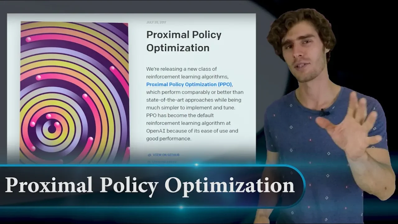

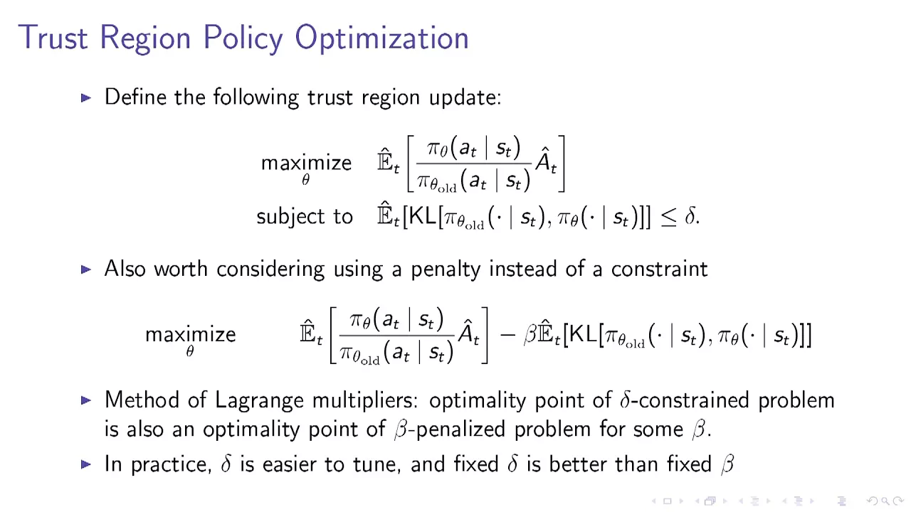



Proximal Policy Optimization (PPO) is an actor-critic reinforcement learning algorithm that addresses the instability problem in traditional actor-critic methods, where small neural network parameter updates can cause dramatic performance drops. PPO achieves stability by constraining policy updates through a clipped objective function that limits the ratio of new to old policy probabilities within a range of [1-ε, 1+ε], preventing large parameter jumps. The algorithm uses Generalized Advantage Estimation (GAE) to calculate state advantages and employs mini-batch stochastic gradient ascent with multiple epochs per data sample. PPO maintains separate actor and critic networks, with the actor outputting action probabilities via softmax activation and the critic evaluating state values. The implementation involves storing trajectories in a fixed-length memory buffer, performing multiple network updates per trajectory, and combining actor and critic losses with appropriate coefficients for optimization.
PPO Implementation With PyTorch | Reinforcement Learning Tutorial
Added:welcome to a crash course in proximal policy optimization before we begin a quick Shameless plug my udemy courses on deep reinforcement learning specifically an critic methods and deep Q learning are on sale right now learn how to turn papers into code Link in the description below so proximal policy optimization or PO for short was created for a pretty simple reason and that is that in actor critic methods often times we see that the performance can fall off a cliff the agent will be doing really well for a little while and suddenly an update to the neural network will cause the agent to Simply lose uh its its understanding of how to play the game and so performance tanks and never really recovers now this happens because actor critic methods are incredibly sensitive to perturbations the reason being that small changes in the uh underlying parameters to our deep neural network the weights for instance can cause large jumps in policy space and so you can go from a region of policy space where performance is good to a region of policy space where performance is bad just by a small tweak to the underlying parameters of your deep neural network po addresses this by limiting the updates to the policy Network it has a number of mechanisms for doing this uh but the basic idea is that we're going to base the update at each step on the ratio of the new policy to the old and we're going to constrain that ratio to be within a specific range to make sure we're not taking really huge steps in um parameter space for our deep neural network of course we also have to account for the goodness of State in other words the advantage how valuable each state is and the reason being naturally that we want the agent to select states that are highly profitable to it over time so it wants to find the best possible States now taking into account the advantage can cause the uh the loss function to grow a little bit too large and so we're going to be introducing a way of dealing with that by clipping the loss function and taking the lower bound with the minimum function something else we're going to be doing that's different than what you may be used to is that instead of keeping track of something like say a million Transitions and then sampling a subset of those at random we're going to be keeping a very small fix length trajectory of memories and we're going to be uh doing multiple Network updates per data sample using minibatch stochastic gradient descent it's noting that you can also use multiple parallel actors on the CPU something like what you would do in a3c but we're not going to deal with that in this particular tutorial I'm just going to show you how to do the GPU implementation so let's talk about the mini batch gradient uh scent for a second so we're going to keep track of a list of memory indices from say 0 to 19 and that's for the case of taking a look at 20 Transitions and let's say we want to take a batch of size five and so those batches could start at position 0 5 10 or 15 uh those are the only uh possible positions where to start such that you get all the memories you don't get any overlap and uh that it all works out evenly so what we're going to do is we're going to shuffle our memories and then take batch size chunks so we'll start at position zero go from zero all the way up to four that is one batch and then position uh five up to 9 is the next batch and so on and so forth It's relatively straight for when you see it in code but it's kind of difficult to explain as you're coding it so just know that we're taking back siiz chunks of shuffled memories for a mini batch stochastic gradient Ascent other things we need to know is that we're going to be using two distinct networks for our actor and our critic instead of having a single network with shared inputs and multiple outputs now you certainly can use a shared input with multiple outputs but it complicates the loss function a little bit and I found that performance is generally adequate with two distinct Networks for simple environments so the critic will evaluate the states at the agent encounters uh and it gets the name critic because it literally criticizes the decisions that the actor makes based on which states it ends up in so it says hey this particular state was valuable we did good or this state is stupid we did bad do better next time now this is in contrast to State and action pairs for something like say deep Q learning but it's in line with what other actor critic methods use and of course the actor decides what to do based on its current state so our network is going to Output probabilities using a soft Max activation and we'll use that for a categorical distribution and Pi torch so we'll have in the case of the cart pole we'll have a couple actions and some probabilities selecting each action and then we will use the probabilities determine bar deep Neal Network to feed into a distribution that we can sample and use for the calculation of the log probabilities more on that momentarily it's also worth noting that exploration is going to be taken care of for us due to the fact that we're using a distribution so it's probabilistic and it's set up so that each element has some finite probability so even if the probability of one action goes arbitrarily close to one the probability selecting the other action stays finite so that at least some of the time it's going to get some exploration this is in contrast to something like say epsilon greedy action selection and deep Q learning where you select off uh off optimal actions about 10% of the time as I said earlier our memory is going to be fixed to a length of capital T in this case we'll use 20 different steps we're going to keep track of the states the agent sees the actions it takes rewards it receives the terminal Flags the values of those States according to the critic Network and the log of the probability of selecting those actions that'll be become important later in our update rule as I said we're going to shuffle those memories and Sample a batch size of five and we're going to perform four Epoch of updates on each batch now these parameters are chosen specifically for this particular environment and that's one of my criticisms of PO is that there are a number of parameters to play with hyperparameters the memory length is one hyper parameter the batch size and number of epoch as well as learning rate and another parameter we're going to see later all play roles of hyper parameters in our model and so there is a lot to tune here but these parameters work really well for the um cart pull environment so you won't have to do any tweaking for that other thing to note is that this memory length capital T should be much less than the length of the episode so in the case of the cart pole the maximum episode length is 200 steps and so 20 steps is significantly less than that so I think it qualifies you wouldn't want to use uh something that enccompass more than one episode for instance um that would probably break the algorithm and result in poorer performance relative to using a capital T much less than the episode length so all this is relatively simple but what isn't so simple is the update rule for our actor so here's where all the math comes in so we have this quantity loss CPI this stands for conservative policy iteration and it's given by the expectation value which is just an average of the product of the ratio of the policy under the current parameters to the policy under the old parameters multiplied by this aat subt on that in a second and they just and they just abbreviate that ratio is R subt now if you're not familiar with deep reinforcement learning or reinforcement learning in general the policy is a probability distribution that is what our actors attempting to model is a probability distribution the policy and this policy is a mapping between state and actions and probabilities so given your inate s subt and you took action as subt what was the probability of selecting that action according to the distribution and so in the denominator we have Theta old that is the um probability of selecting action a subt given State s subt uh under the old parameters of your deep neural network so we're going to play 20 steps and then the agent is going to perform a learning update and it's going to do a mini batch stochastic gradient ascent and so after Computing that first batch the parameters of the deep neural network change right that's how the uh batches work you compute the loss with each batch and update your parameters and so right after you've calculated that first batch of memories the loss for that and updated your deep neural network uh the Theta changes and so the policy Pi is going to change as well so we have to keep track of the parameters uh excuse me of the the probabilities uh of selecting each action at each time step in our memory and then on a learning function we're going to pass those States through our actor Network get the probabilities the probability distribution and find out what the probability selecting action a subt is sampled from our memory according to the current values of the deep neural network it'll be a little bit more clear in code uh just know that we have to keep track of log probs as we go along and we're going to be recalculating them in the learning Loop one thing we also see is that it takes into account the advantage which is at a hat subt so the advantage is just a measure of the goodness of each state we'll get to the calculation of that in a few minutes uh but one thing to note is that this ratio uh Pi sub Theta over Pi sub Theta old um can have an arbitrary value right because you could have let's say Pi Theta being.99 Pi Theta old 01 and so that's a pretty large number and in particular if you multiply it by an advantage that is like say 10 20 whatever then that can also still be a large number and so we have to deal with that right because the whole point of this is that we want to constrain the updates to our deep neural network to be some relatively small amount and so the way you deal with that is by adding an additional hyperparameter Epsilon that you use to clip that ratio so what we're going to do is we're going to clip that ratio within the range 1 minus Epsilon to plus 1 plus Epsilon so let's say from 0.8 to 1.2 so that ratio is going to be constrained to be close to one and you're going to multiply that by the advantage and so that'll give you some number and then you want to uh take the minimum of that clipped number the clipped ratio multiplied by the advantage and the unclipped ratio multiplied by the advantage take the minimum and that is what we will use for the loss for our actor Network so this serves as a pessimistic lower bound to the loss and they don't go into any real depth in the paper on the reasoning for this uh but to my mind and this could be wrong you know I am an idiot sometimes but my understanding is smaller loss smaller gradient smaller update that's the whole point of it so let's talk about this Advantage now so this Advantage um has to be calculated at each time step and it's given by this equation now don't freak out this is relatively straightforward uh once again it tells us the benefit of the new state over the old well how do we know that we know that because it's proportional to or equal to the sum of the Delta subt where the Delta subt is just the reward at a time step plus the difference in the estimated value of the new state and the current state so it tells you what is the difference in the value between the next bet the next state we encounter and the current state and of course you have the gamma in front of the V which is the output of the critic Network because we always discount the values of the um next States because we don't know the full dynamics of the environment and so the that reward is uncertain there's always some uncertainty around State Transitions and then in the top equation you just sum that uh where you're going to be summing over gamma multiplied by Lambda so uh this quantity gamma is again the normal gamma 0.99 that we typically use but this parameter Lambda is a type of smoothing parameter it helps to reduce variance and we're going to use a value of 0.95 and for implementation we're just going to use uh a couple of nested for Loops so you're going to start out at time T equals 0 and then Su from that step all the way up to capital T minus one so if we have 20 States you're going to go from zero to uh capital T minus one 0 to 18 and you have to do that because you have the V of s subt + 1 you don't want to try to evaluate something Beyond uh the number of actual states that you have that won't work out right um and so it's going to be relatively straightforward once you see it in action and we're going to be keeping track of that gamma time Lambda which is a multiplicative constant that increases its power by one with each iteration of the inner loop all that'll be made clear in the code uh but fortunately the critic loss is a little bit more straightforward so we need something called the return so um the return is just equal to the sum of the advantage and the critic value based on the memory so whatever the agent estimated the value of a particular state to be at the time that it took it is what we're going to be using for the critic value in our return and then the loss of the critic is just going to be the mean squared error uh between the return and the critic value based on the current values of the deep neural network so once again we're going to be passing the states through the critic Network to get its estimate of values and we're going to be also using the values from the memory as well so relatively straightforward even easier when you see it in code so we have two different losses and we have to sum them and so that'll be the sum of the clipped actor and critic so a couple things to note here is that one we're actually doing gradient ascent and so the coefficient of C1 for the loss of our um critic is going to be positive and uh the um loss of our is going to be negative because we are doing gradient ascent and not gradient descent we have to multiply by negative 1 other thing to note is that we have this other parameter here C2 this coefficient multiplied by s s is an entropy term and that only comes into play when you have a deep uh neural network with shared lower layers and actor and critic outputs at the top so we don't have to worry about that in our particular implementation in this tutorial because we're doing two separate networks for the actor and the critic and I'm going to use a coefficient of 0.5 for the um loss for the critic as I said we're not going to be implementing the entropy term because we're doing two distinct networks um we can also use this for continuous actions there you would use a different output for your uh actor network uh and indeed that's what the paper really is geared for is for continuous action spaces but we're going to be doing the very simple discret case other thing we won't Implement is the multicore CPU implementation because that introduces even more complexity we're just going to be using the GPU so what do we need for this project we're going to need a class for the replay buffer and we're just going to use lists for this normally I like to use numpy arrays but in this case lists turn out to be a simpler implementation so that's what we're going to go with we're also going to need a class for our actor Network and a class class for the critic Network we'll need a class for agent that's going to tie everything together that'll have actor and critics that invoke actor and critic uh Constructors as well as a memory uh for storing the appropriate data it'll also have functions for choosing actions storing memories saving models and learning from its experiences and in a separate file we're going to have a main Loop to train and evaluate the performance of our agent before we get into the coding section I want to do a quick shout shout out to William Woodall he hangs out in our Discord Channel which is also linked in the description below if you want to come hang out uh with some really really smart people who talk about uh artificial intelligence ranging from all sorts of different things every single day check the link in the description for the Discord so William came to me and said hey Phil I found an implementation of Po that I find to be in line with your general philosophy of software minimalism and he showed it to me and I looked at it and it helped clarify quite a few questions I had after reading the paper now the software you see here is pretty much my own code but it was inspired by William woodall's code so shout out to him for helping me out on this because the paper really isn't all that clear to me um even after reading it a few times other thing I want to say uh and I'll talk a little bit more about this in the coding section is that when I normally define deep neural networks actors and critics in particular I will use the convention of saying self layer name equals nn. linear uh self. layer name next you know equals nn. linear and then I'll write the feed forward function where you use the um member variables that self. layer one as something you can call as an object to call and then calling activation functions within that now what I found is that doesn't really work very well in fact I have to use nn. sequential to create the models for this and that's one of the biggest takeaways I had from William woodall's code is that uh by using the nn. sequential you really get this thing to work and for whatever reason I cannot get as good a performance using my conventional typical way of writing these networks now that I can't think of any reason why that should be the case but it is something I've observed I tested it uh just altering that one chunk of code how I Define the models and running it several times to take into account run to run variation and it seems to be repeatable for me so maybe I don't know maybe it's a configuration issue on my system maybe it's something I'm doing wrong elsewhere I don't know I don't think so all of that out of the way let's go ahead and get into the coding portion all right so let's go ahead and jump right into it with our Imports they're going to be pretty light we'll need OS to handle file joining operations numpy for numpy type stuff and all of the torch packages we'll need and then for our sequential model we will need optim and we will also need our categorical distribution so we'll start with our po memory class and this will be pretty simple for the most part the only input for our Constructor is a batch size and we will just implement the memory with lists so we'll keep keep track of the states encountered the log probs I'll just call it probs for brevity the values that are critic calculates the actions we actually took rewards received and the terminal Flags so next we need our function to generate our batches so our strategy is going to be the follow following we're going to have a list of integers that correspond to the indices of our memories and then we're going to have batch size chunks of those memories so indices from zero to say four and then five to 10 so on and so forth or whatever our batch sizes we're going to shuffle up those indices and take those batch size chunks of those shuffled indices so the first thing we need to know are the number of states we are going to want to get our batch start list or array I suppose that'll go from zero to n States in batch size steps batch size it would help if I could type our indices and that is just the number of states in our trajectory um we're going to want to shuffle that so that we handle the stochastic part of the mini batch stochastic gradient ascent and then we can go ahead and take our batches using a list comprehension so it's going to be those indices from I to I plus self.
batch size for I in range for I in batch start so it's going to take all of the possible starting points of the batches either 0o 5 10 Etc and go uh in the indices from that all the way up to I plus batch size so we're going to get the whole batch from our indices and then we're going to want to return an array for each of those and this gets a little bit messy and I have to be very careful not to mess up the order because of course the order in which you return the memories definitely matters later on we'll need Rewards and then we're also going to want to return the batches and the reason why will become apparent later uh it's because we're returning the entire array here and we're going to want to iterate over the batches so now we need a function to store a memory and that'll take a state action probability value reward and done as input and all we're going to do is append each of those elements to the respective list that is reward singular and then finally we need a function to clear the memory at the end of every trajectory and I forgot the self argument here and mini rant here I really don't like some aspects of python uh it took me much longer than I would care to admit to get this to run not because the algorithm I implemented was incorrect but because I had a mismatch so here I had I believe action and up here it was actions or perhaps vice versa in my original implementation so it didn't flag as an error uh because it's not really an error particularly where python is concerned and uh uh so it was quite a nuisance uh pretty pretty painful to track that down um of course it were a more strongly typed language then that wouldn't be an issue but I digress so now let's handle our actor Network and and that will derive from the base nn. module class our initializer is going to be pretty straightforward for actor we will need the number of actions the input dims Al learning rate Alpha number of fully connected dims for the first and second fully connected layers and a checkpoint directory and we're also going to need to call our super Constructor and then create our checkpoint file checkpoint directory and actor torch poo now I do it this way because I'll often do development in a single root directory and I don't want to get models mixed up if you have a different way a more organized way of writing software then you could perhaps skip this path joint operation and just use a file by itself but let's move on to the actual deep neural network uh we're going to want a linear layer that takes star input dims so we're going to unpack the input dims so we have to pass in a list and it's going to Output fc1 dims a relo activation function another linear layer that takes fc1 dims as inp put outputs fc2 dims that gets a rue activation as well another linear layer that takes fc2 dims as input and outputs a number of actions and then we're going to use a soft Max activation along the minus1 uh Dimension so that's the whole of our actor Network the softmax takes care of the fact that we're dealing with probabilities and they have to sum to one so our Optimizer is going to be an atom Optimizer what are we going to optimize the parameters with the learning rate of alpha of course we need to handle the device which would be our GPU if possible then we want to send the entire network to the device next we have our feed forward function and that'll take a single state or batch of States as input so we want to pass that state through our NE deep neural network and get the distribution out and then use that to define a categorical distribution which we are going to return so what this is doing is it is calculating a series of probabilities that we're going to use to draw from a distribution to get our actual action and then we can use that to get the log probabilities for the calculation of the ratio of the two probabilities in our update uh for our learning function then we have a couple of bookkeeping functions save checkpoint uh we're going to want to say torch.
saave State dictionary for our Network and we're going to save that into a checkpoint file then we need a load checkpoint and that is self. loadad State dictionary what are we going to load a checkpoint file and that's really it for the actor Network it's pretty straightforward uh the critic network is also straightforward and that also deres from nn.
module here we don't need the number of actions because the output of the critic is single valued it just out puts the value of a particular state so it doesn't care how many actions there are in the action space but it does need a learning rate Alpha it does need some Dimensions 256 and a checkpoint directory and then we need to call the super Constructor and same deal with the checkpoint file um the checkpoint directory and critic torch so that way we can differentiate between the actor and critic model files and we will again use a sequential model and so uh in the shout out I was talking about William woodall's implementation as well as something else I observed so what I meant by the alternate method of doing a model was if you say self. fc1 and in linear you know if you do it that way have fc1 fc2 the separate layers defined without the sequential model it actually does significantly worse than if you do it with the sequential model and I don't know why I don't have a certainly there's no theoretical reason it should do it it must be something under the hood with the way in which pytorch is implementing things and uh it's no disrespect to the creators of pytorch but this is one of my you know one of my biggest gripes with using these third party um libraries is you never know how they're implemented so something doesn't operate the way you expect you can certainly go look it up it's open source but that is much easier said than done right you have to be familiar with not the entire codebase but a really significant portion of it to be able to make sense of a single file or a single way of doing doing things so it really makes things opaque it's an abstraction on top of an abstraction um and so I don't know it's part of the good uh part of the it's the bad that comes with the good for having you know a robust Library like P torch but I do it this way because it seems to work the best and as an aside I also can't get it to work very well in uh tensor flow to and I suspect the the reasons are related because the performance of the tensor flow to is on par with the type of performance I get from doing it uh the other way where you just Define individual layers instead of a sequential model so pretty interesting stuff maybe one day I'll get super motivated and decide to go ahead and figure it out but I wouldn't hold my breath on that so this is going to be a very similar model linear layers with radio activations in between the main difference is that our output layer is going to be a linear layer with no activation and a single value output now of course it handles the batch size automatically so if you pass in a batch you're going to get a batch of outputs as well again we need our Optimizer with learning rate of alpha as an aside about the optimizer um I'm going to use the same learning rate for both the actor and the critic and it's entirely feasible and possible and perhaps even advisable to use separate learning rates for both the actor and the critic uh at least in something like deep deterministic policy gradients you get away with a much larger you know by a factor three or so learning rate for your critic than you do the actor uh reason being as we outlined the lecture the actor is much more sensitive to changes in the underlying parameters of its deep neural network U now ostensibly or theoretically the the PO method should account for that and allow you to use uh a similar learning rate because the actor should be less sensitive than in the case of ddpg but I haven't tested it so one thing you can do in your spare time is play around with differing learning rates for both the actor and the critic our Ford feed forward function is pretty straightforward you want to pass a state through your critic Network and return that value and we're going to need um saving and loading checkpoints I am just going to yank and paste those because the functions are otherwise identical and so that is it for our two networks now we come to the heart of the problem problem which is the agent class do I have an extra yes I do and this of course does not derived from anything this is our base agent class we need number of actions a default value for gamma which is the discount factor in the calculation of our advantages typically we use something like 0.99 a learning rate of 0.0 3x 10 minus 4 uh I get this from the paper so um if you read the paper they do give you the hyperparameters and a little bit of detail around the networks they used but it is not a very well-written paper it's rather obtuse um so I'm not a huge fan of it uh but uh we do have some good default values from it so a policy clip so in my sheat sheet here I have a value of 0.1 is a default um although in the paper they use 0.2 perhaps I was experimenting I will have to be careful with that a batch size of 64 a default n of 248 so that is the Horizon the number of steps before we perform an update and the default for the number of epoch now these parameters come from um these parameters come from the values for um continuous environment so the actual numbers we're going to be using are going to be significantly smaller as I said we'll use an N of 20 uh three Epoch batch size of five instead of 64 and I'm going to go ahead and set that policy clip to 0.2 uh now that I'm looking at it we need a GAE Lambda that is the Lambda parameter but of course you can't use Lambda because it is a reserved word for python what else do we need um yeah I think I'm missing something in my other file here that's okay I'll fix it on the fly so then we go ahead and save our parameters uh number of epoch and our GA Lambda need our actor Network input dims and learning rate takes input dims and alpha bbo memory batch size input 1 second all right hopefully that is not as loud now uh the toddler is playing with his grandparents always a hoot so now we need a function that handles the interface between the agent and its memory um and it's just going to be very simple self-memory store memory it's just an interface function then we need a function to save our models uh print saving models that is just going to be an interface function between the agent and the save checkpoint functions for the underlying deep neural networks and very similar for the load models function now we have a visitor all right that is it for our bookkeeping functions next we need something to handle choosing an action that'll take an observation of the current state of the environment as input and we want to convert that numpy array to a torch tensor and we're going to add a batch Dimension because the Deep neural network expects a batch Dimension and we'll be sure to specify that it is float and then we're going to go ahead and pass that through our neural networks so dist equals self. actor State that'll give us our distribution for choosing an action we need the value of that particular State and then to get our action we just sample our distribution uh and then what we want to do is go ahead and squeeze to get rid of those bash dimensions and this might be something I added uh for tensorflow 2 I'm not I don't remember if torch requires it but it doesn't hurt anything so for the problems we want to go ahead and return the log probability of the action we actually took item so do item will give you an integer and likewise for the action we want to squeeze it and get the action the item out and similarly for the value and then just return all three so this will make our main function look a little bit different than we're used to because we're going to be accepting three values from our choose action function instead of one uh but that's necessary for keeping track of the probabilities and values as well next we come to the meat of the problem so to speak our learning function so we want to iterate over the number of epochs so we're going to have in this case three epochs at the top of every Epoch we want to get our arrays the old probabilities the values the reward the D and the batches let's do that um and then I'm just going going to use a different notation here and go ahead and start calculating our advantages so our advantage is just going to be a numpy array of zeros L reward type MP float 32 and we're going to say for T and range so for each time step Len of reward array minus one because we don't want to overwrite the or go beyond the bounds of our array our discount factor is going to be one the advantage at each time step starts out as zero so we're K and range so we're going to start out at T and go from T to the same reward array minus one and say as subt plus equals discount so that GAE time Lambda Factor uh which starts out as one times we need parentheses reward array subk plus self.
gamma times values k + 1 times [Music] um one minus int done array K minus values subk then we say discount times equals s. gamma time GA Lambda and at the end of every calculation the end of every K steps Advantage subt equals at a subt and at the end we're going to turn advantage to a tensor in particular a Cuda tensor and this is just a strict implementation of the equation from the paper so this uh right here in parentheses is the Delta subt so it's a reward plus a gamma * V subt + 1 minus V subt or you know we swapped k and t here um and you need the one minus duns uh on the values as a multiplicative factor of the values of T sub t + one because the value of the terminal state is identically zero that's just a convention in reinforcement learning it it predates the Deep neural network stub is just how we handle it it's assumed that's why they don't put it in the calculation it is assumed it's just a matter of convention and then that discount is the GAE the Lambda multiplied by the gamma that takes care of the multiplicative Factor so it is the the gamma Lambda to the uh T minus one power or is it T minus K minus one something like that power multiplied by the Delta and then you're summing it all up so now we have our advantage um I'm going to convert the values to a tensor as well and I fully admit here that going from vals array to you know what in fact let's do this no let's leave it the way it is uh may not be the most uh effective or excuse me the most uh efficient way of doing it but sometimes I just get stuff to work and then don't go back and clean it up if you want to clean it up please do so I always invite that and it looks like I'm missing something here because it is um not automatically indenting so I'm probably missing a parentheses somewhere and it is right here I believe if I am not mistaken yeah there it goes all right so then States is just going to be a tensor State array subbatch D type T.F float to sal. actor.
device and we're kind of violating the pep8 style gu style guide by going Beyond 80 characters but I think we'll be all right old probabilities gets converted to a tensor and I don't need an explicit D type there I don't think do device.
two self. actor device that works and then actions okay and then um so we have the States we encountered the old probabilities according to our old actor parameters the actions we actually took uh the next parameter we need so we have the bottom of that numerator Pi Theta old we need Pi Theta new so we have to take the states that we encountered and pass them through the actor Network and get a new distribution to calculate that new those new probabilities and we'll also need the uh value of the the new values of the states according to the updated values of the critic Network so we may as well get those now and we can squeeze those and then we can calculate our new probabilities and take the prob ratio so here I'm going to exponentiate the log probs to get the probabilities and take their ratio you could also do this those two are equivalent by the properties of exponent uh exponents um exponentials excuse me and then we're going to calculate our weighted probabilities and sorry our probability ratio um no yeah the weighted probabilities I think I have two lines that do the same thing in there that's funny and that's going to be the advantage uh batch times a probability ratio then we need the weighted clipped probabilities and that is going to be the clamp of the prob ratio between one minus self do policy clip and one plus self.
policy clip multiply by Advantage sub batch now our actor loss is going to be the um negative minimum of the weighted probs or the weighted clipped probs mean and our returns for our crit Closs are going to be the advantage plus the values for that particular batch and so our critic loss then is going to be the returns minus critic value squared and the mean value our total loss at loss plus 0.5 time critic loss remember we're doing gradient ascent and there's a negative sign in front of the actor um so we're not doing descent that's another thing that's kind of suboptimal by the way the paper is written uh you can get kind of confused about negative signs if you're not paying very careful attention next we have to zero our gradients I think you can probably hear that my son is giving a concert downstairs he's playing the drums by whacking on his toy box with some drumsticks um so we're going to back propagate our total loss and then step our optimizers and finally uh at the end of every Epoch yeah I think that's the right indentation we want to clear our memory so at the end of all whoops at the end of all the epoch we want to clear our memory let me just make sure I'm not doing that egac no I am not okay that is good so now let's do a right quit and I have an indentation error here I see oh that came when I did the uh yank and paste all right so that is it for our um agent file let's go ahead and take a look at Main so we start with our Imports we'll need gy we'll need numpy to uh keep track of the running average of our scores from po torch we'll need our agent and if you're new here I have a utility file that I use a map plot live P plot function to plot the running average of the previous 100 games for the learning curve it's pretty trivial you can just do a plot of the running average um just do a get clone if you want to use my exact version I don't go over it in every video because it's kind of redundant but I leave a link in the description to the GitHub so um go ahead and do a a clone of that so you have that file or just write your own so we're going to use the very basic cart pole v0 uh reason being uh we don't need to spend a whole lot of time on a very computationally complex environment to realize we made a mistake so it's very easy to see if something got screwed up with the cart pole environment this certainly will work on more advanced environments but it does require a little bit of um fine-tuning so uh we'll just start with a cart pole and then you can play around with other environments at your leisure so we'll use the parameters I dictated in the lecture I think I change the number of V box to four running rate of three we can get the number of actions directly from our environment very handy uh pass in all the other relevant parameters get the number of input Dimensions from our environment and we're only going to play 300 games as I'm looking at this I do realize that um in the parameters I did the last time I ran it I did do a policy clip of 0.1 but 0.2 comes from the paper and I'm I'm pretty sure it works both ways so we will find out if we need to we can go back and change the policy clip uh not a big deal so plot cart poole.
PNG we need to keep track of our best score this minimum score for the environment empty list for our score history and um number of learn times we call the learn function you can make this a member variable of your agent if you want and an average score starting out of zero we don't actually need that but whatever so we'll say at the top of every episode to reset our environment set the terminal flag to false and cumulative score to zero while we're not done we need to choose an action based on the current state of the environment um get the new state reward done and debug info back from the environment increment our score by the reward and store that transition in the agent's memory reward and done and if n oh I do need an extra variable here we'll say in steps equals zero and that's a number of steps we take and we need that because we have to know how often or when it's time to to perform the learning uh function so every time we take an action the number of steps goes up by one so end steps modulus n equals z then agent.
learn it plus equals 1 and then no matter what happens we want to set the current state to the new state of the environment and the end of every episode append our score and calculate our mean and that's the previous one 100 games if that average score is better than the best known score then set that best score to the current average and save your models and we also want some debug information is so I score of course that should be an average score the uh I like to print out this isn't necessary but but the number of steps that have transpired in total and the number of times the agent has called The Learning function this gives you an idea uh this is I did this because when I compare with the results of the paper um it wasn't clear to me if they were talking about the number of times they called The Learning function or the actual absolute number of uh time steps in the environment uh so I print out both this time steps and learning steps are totally optional you don't have to print it out it's not something that is required so I just do it for my own clarification we need an x-axis for our plot lens score history and plot learning oh certainly let's do this we don't want to do it every single game we want to do it at the end of all games all right now moment of truth let's see how many typos I made so it's telling me in it got an unexpected argument input dims that's interesting what do I call it I don't have it there no and the reason is my computer had a hard lock up and I had to do a reboot and it mutilated my cheat sheet for this so there bound to be some errors in here ah I didn't do my make directories so temp Po and plots let's try it again name duns array is not defined it's probably done array that is in line [Music] 161 so it is dun's array yeah we'll just change it there I guess old prob array is not the that's probably the same thing uh where am I yeah old prob array and I'll do the opposite here I'll make it singular just for just for the sake of not being consistent index 8 is out of bounds okay so then something has gone extremely wonky with the generation of the batches um okay let's take a look at that oh wait let's read this a little bit more carefully it says index 8 is out of bounds for axis Zer with size zero so our action array oh you know what let's take a look at our memory so it's action array so here we have self.
actions uh we return the self actions self dot ah there we go that's why so actions.
append action all right now let's try it name Advantage is not defined that is a typo that is in Line 183 a Advantage did I yeah let's try that let's try once more has no memory underscore clear memory that's memory do clear memory 197 all right so now it is running so I'll let that go for a few minutes and we will see how it does all right so it has been running for a little bit just a few minutes now it runs relatively quickly and what I'm seeing is that we do get some oscillations in performance you see It'll hit 200 for you know several games in a row and then it'll drop down into the mid 100s even you know 66 something relatively low like that and there's a little chunk here where it dips below 100 points so uh it's not a silver bullet but it looks to be be recovering so we'll give it another 80 runs and see how it does okay so it has finished up and you can see that it finished strong with a long run of about 50 games 45 games of a score of 200 so uh I commented when I was writing the agent that I was looking at my cheat sheet and had a policy clip value of 0.1 it could be that I had settled on that value based on some experimentation um and then changed it back just to be more consistent with the paper for this particular video uh so that's something I would play with uh other thing to consider is that there is significant runto run variation that is a facet of pretty much every algorithm in deep reinforcement learning it just has to do with the way the neural networks are initialized as well as how the uh number random number generators initialize the environment so um when you see papers they'll typically report uh average values for say five or 10 or whatever number of games and then a band to show the range of variance for runto run variation uh but this is clear evidence of learning you know it achieves a score of 200 and under 300 games uh so I call this good to me this is fully functional now there are a number of things you can do to improve on this you can get it to work with continuous environments you can bolt on uh some stuff for doing um Atari games where you would need to add in convolutional neural networks uh as your input layers and then flatten them out to pass them to a uh linear layer for the actor and the critic and you can see my earlier video on an AI learns to beat pong for q-learning there I go over all of the um a lot of the stuff you need to do to modify the open AI gy Atari environment uh to do frame repeating that's something they do in q-learning uh that's an exercise to the reader um actually I don't know thinking back to the paper I don't recall if they actually do any frame repeating or not in this particular algorithm poo uh but it's just something to look at anyway uh so there's a number of things you can do to improve upon it I haven't added this module to my course yet I'm still working on it I really want to uh take some time to give more thought to the paper because the paper isn't very well written and I'll probably have to do a lecture like what I did for uh this YouTube video in the course because the paper isn't very easy to implement just by reading it so I hope that was helpful that is Po in just a few hundred lines uh full implementation in pytorch solving the C pole environment then you can easily modify this to do other environments As You Wish if you've made it this bar please consider subscribing hit the Bell icon leave a like a comment down below and I'll see you in the next video
Up Next
Deep Q-Networks: Reinforcement Learning with Neural Networks
@aiprism1155
39.3K views•2017-10-05

Secure Multiparty Computation (MPC): Foundations & Challenges
@SimonsInstitute
7.3K views•2015-05-28
Create Your Own Reinforcement Learning Environments: Gridworld Tutorial
@MachineLearningwithPhil
39.1K views•2019-04-02

Neural Networks Explained: Math, Layers, and Learning Fundamentals
@3blue1brown
21.9M views•2017-10-05
Related Study Plans & Knowledge Roadmaps
Structured learning paths in Artificial Intelligence