



![[Python] أساسيات البرمجة باستخدام لغة بايثون](https://i.ytimg.com/vi/sBh4vNcIPkQ/maxresdefault.jpg)





















This tutorial demonstrates how to build a basic neural network using Keras in Python, covering the Sequential API for model creation, dense layers for feature extraction, flattening input data, softmax activation for multi-class classification, and training with epochs and batch sizes, while explaining key concepts like hyperparameters versus trainable parameters and the importance of validation data to prevent overfitting.
Building Your First Neural Network with Python and Keras
Added:Basic Python programming proficiency, including data structures, control flow, and functions.
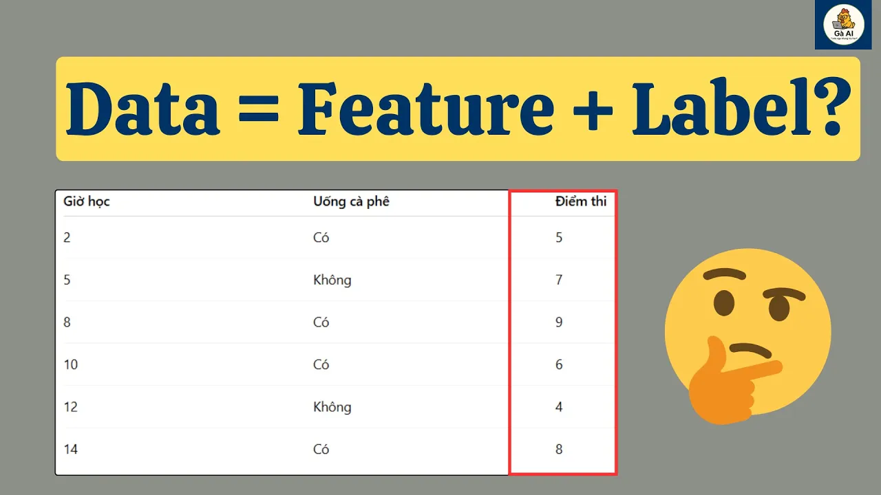
Foundational understanding of machine learning concepts, such as supervised learning, features, labels, and the split between training and testing data.
Familiarity with the NumPy library for handling multi-dimensional arrays and performing basic mathematical operations.
Basic mathematical intuition of linear algebra (matrix multiplication) and calculus (gradients and derivatives).
Exploring specialized neural network architectures, such as Convolutional Neural Networks (CNNs) for image processing and Recurrent Neural Networks (RNNs) for sequential data.
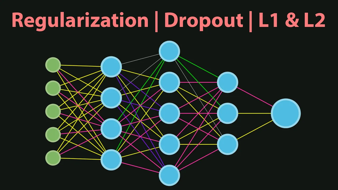
Implementing regularization techniques like Dropout, L1/L2 regularization, and early stopping to prevent model overfitting.
Advanced hyperparameter optimization strategies, including learning rate scheduling and systematic grid or random search.
Deploying trained Keras models into production environments using frameworks like TensorFlow Serving, Flask, or FastAPI.
10.6K views227likes18:00Original Release: 2022-10-14
Now it's time to build the first ever neural network.
So as I said, we're using us.
Um, we, as you see here, what we do is very, very simple.
Actually, we're just creating a model and we are adding layers, layers to it.
So basically model add a Cara Slayer model, add a Carol Slayer model, add a Carol Slayer.
So it's quite simple.
Um, In theory, but of course you can go as deep as you want.
So let's start with the first line we have model model equals two care us models.
Sequential.
There are three ways how you can create models with Kara.
So you have this quite sequential class, which is very simple.
You just choose the predefined layers and then put layers on top of.
Uh, there is a functional class, which is a little bit more detailed.
You can create more complex, uh, neural networks with that one.
Uh, but we don't need the functionality now.
So we're just using the simplest one.
There was also a model, uh, models library inside.
And before that one, you basically make everything from scratch manually.
And that is more for if you're doing research and if you're trying to achieve the highest possible a curiosi, uh, and that's not really something that we need here.
All right.
The second line here is a layer that we're.
And the first layer that we're adding is basically the input layer.
What is done here.
And the flattened layer is because we have a 28 to 28 matrix.
We want to make it one big string of 784 pixels.
That is 28 times 28, 784.
And I am saying the input shape is this much.
Please flatten it.
And flattening.
It means that adding them one after another, making it one long line, and that is a number of inputs.
Topic going.
The next line we are creating actually the next two lines we are creating hidden.
Uh, hidden layers or cold dense layers here.
Well, not specifically hidden layers, but older layers are called dense layers.
That means they are connected with everything that is before them or after them in a dense way.
So you might see here this word and other places do either, do you have dense and sparse dense means every neuron is connected to every other.
Sports means not every neuron is connected to every other neuron.
So there are some missing links in between, and sometimes you need that too, but we will talk about that in the future lessons.
So right now, all we need is dense layers for the second hidden or the first hidden layer.
I have a 300 neuron layer and I'm going to keep the activation very low because as we talked about, as we mentioned briefly in the previous lessons about the building blocks of neural networks, value is one of the best ones that we can.
Especially for hidden layers.
Same for the second hidden layer.
We have hundred neurons and we are setting the activation to be with.
And the last one is our output layer.
Actually we have 10 output layers.
And why is that?
It's because there are 10 classes and you want to classify our images, the input images into 10 different classes.
So that starts from zero to 1, 2, 3, all the way to nine.
And that makes 10 different classes.
And we want our model to make a prediction for each of these classes.
So every time they give it, an image is going to tell us how likely it is that it says zero.
And then how likely it is that.
And so on and so forth and also how likely it is that it's a nine and at the end we will have, uh, the possibilities.
Oh, which number this image is here.
Uh, you might realize that we were using softmax softmax, I'll just quickly show you what it looks like.
So it looks like this, it goes from zero to one.
And in that case, it looks very similar to six.
Uh, but then you can ask, why are we using soft max and not signaling because in this exercise and this problem specifically the classic.
Uh, I not related to each other, so they cannot, one image can not be half, one and half the other.
They are completely in the, in the independent.
Yes.
And, uh, what Sigma does is it creates possibility that creates probabilities that are independent from each other.
Same thing can have 0.5 possibility to be two different things.
Whereas for softmax all the possibilities of summation of all the possibilities and.
Lead to one.
So they sum to one.
So that means that if something possibility of an image being two is higher, that means possibility of it being three needs to be lover.
Uh, and that's, that's the kind of thing we need because the images we give can only be one thing.
They cannot be multiple.
Uh, and that's why we're using softmax.
So once we build our model, we can look at a summary of our model.
Um, so this is a nice little function that tells you what your model looks like.
Uh, let's see.
So, as I said, the flattened layer, the input layer has 784.
The dense layer has 300 neurons.
Uh, the first hidden layer, the dense too, you know, they cannot cope be called the same thing.
So that's why they have, they underscore one underscore to the first hidden layer.
It has 300 neurons.
The second hidden layer has hundred neurons and the output layer has 10 neurons.
And for each of these, we also have the number of.
And also we have a total number of parameters.
And what are these parameters?
As I said, for every connection between two neurons, we have the weights and for every neuron itself, we had the bias.
So in total we have a lot of parameters and what our model is going to do is update.
Uh, weights and biases to give us the best security possible.
And if you want to do it, you can also take a look at what your layers look like.
So Kara is basically has a lot of, um, nice functions or commands for you to look into the model that you built.
Of course, it's not always going to be the simple, you know, you're going to build something more complex sometimes, and you might need to look at some summaries or look into the layers and see what your.
The next thing that we want to do is to compile this model.
So it was.
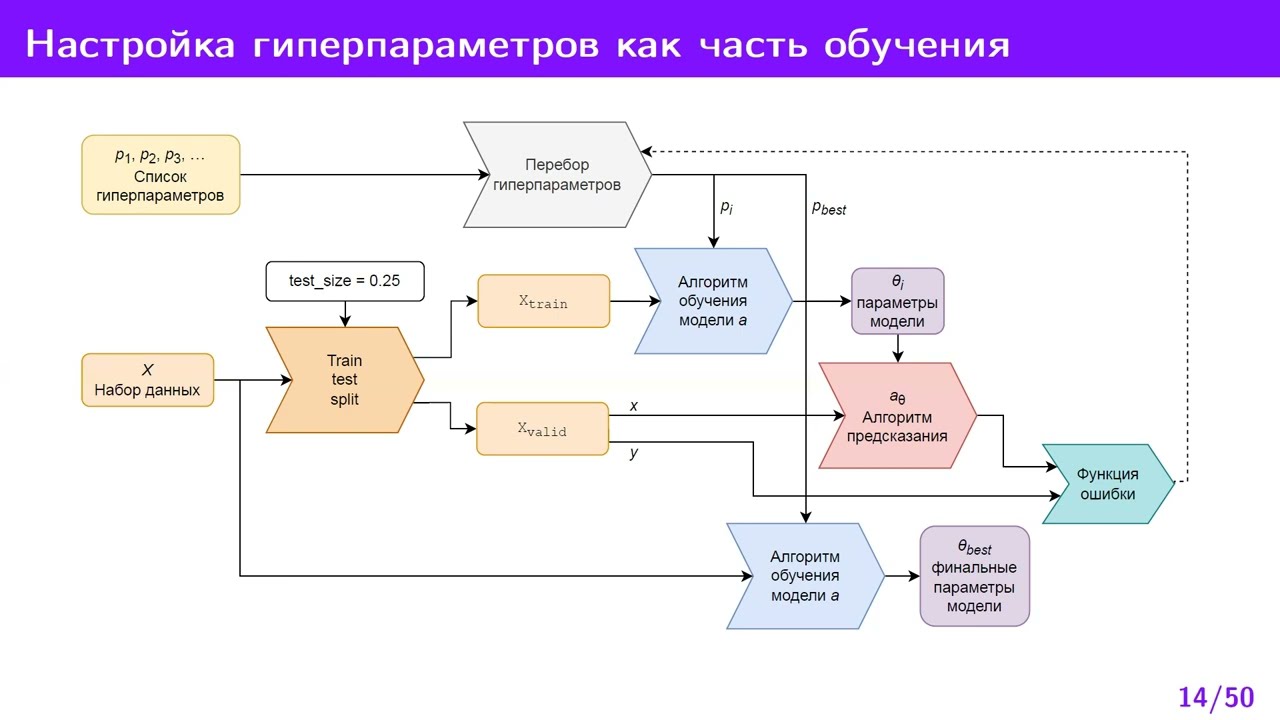
What we're doing is we're basically giving it some hyper parameters here and hyper-parameters are things that you have to set yourself beforehand.
They can not be learned.
So parameters, as you see here are things that going to be learned is also says trainable parameters.
These are all going to be learned.
So they're going to either be initialized to zero, thus for.
Or they're going to be initialized, randomly that's for weights.
Um, but on top of that, while you're compiling your model, you also give it some, uh hyper-parameters.
So these are things that you basically hard-code, and that are not going to be changed.
Um, all of these options.
You can actually see for all of these things, but options that you have.
So for example, for loss, for using sparse categorical cross entropy, and that means that is this thing, spar, sparse, categorical cross entropy is how we're going to measure how good our model is doing.
So, uh, you have some other ones too, so let's go here.
I'll, I'll show you some other options.
So for everything basically on Cara's, you can.
Uh, see what options you have.
So it's says poor, realistic losses, aggression losses.
After a while of working with deep learning or generally machine learning, you'll probably have an idea which one to use.
Uh, but generally, if you don't have an idea, you can Google for it or you can come and look here at the, uh, options.
So let's go and find the one that I'm using right now.
Sparse, categorical, cross entropy.
And it says, use this cross entropy loss function when there are two or more labeled classes.
And that's what I have.
I have more than two label classes right now.
And that's why I'm using suppress categorical cross entropy.
Uh, but as I said, based on your problem, if it's a classification regression problem, or what do you want to get out of it and the type of output that you're getting, you're going to want to change this.
Of course.
Uh, but yeah, we will talk more about these in the future.
Uh, optimizer.
We are using a stochastic gradient descent.
Again, you can find the available optimizers here.
Let's take a look quickly.
So we have this one, the gradient descent, one AIDEM ADA, grad, ADA, max, Natum all of these things.
Um, of course these are not only made randomly these choices.
So right now we are using gradient descent because that's kind of like the basis one that you use.
But if you want to make your model faster, for example, you can use some other things.
But as I said, we will go take a more systematic look on which one to choose.
And when, uh, in the coming.
The last one is the metrics.
This is basically what you want your model to report on while it's training.
So you don't only want to see the loss of reported.
If you want to see some other things reported, you can also add them here and then your model will report it for you.
So let's compile this model and, uh, I don't need this one.
No, yes.
So the last thing that we are going to do is basically.
The model around our data.
And that's why here we have the training, uh, X and Y values for the training.
And we have some other things I'm going to explain.
Um, the one thing that you might want to know again, here is a website where you can see.
What are the options of things that you want to set?
So here you're seeing I edit the datasets, the X and Y value for the dataset, what the model is going to fit on.
But on top of that, I am setting the airbox validation data and that size, these are not the only things you can set.
Of course you can set all of these things.
So right now I'm giving X and Y I'm giving size.
I'm giving ebox, I'm also giving validation data, and these are.
All the other things that you can still set now, we don't need to do them right now, but you can come here and read what they all mean.
So for example, my bows would mean, give me more information about what's happening while the, uh, the model is training.
Um, or for example, instead of giving the validation data here, specifically, we can say validation split and say like this validation spit, uh, equals 0.1.
So.
The model for set asides is a 0.1, 0.1 of the whole training set aside to use as validation data.
So you don't have to do the split beforehand.
Um, so these are all the options that you can have things that you need.
You don't need to use them right now, but you know, just in the future, if you want to check it out and also these values that you see here as equal are the default values.
So if you don't specify it, this is what it's going to be like.
So if you don't specify the epoch, it's just going to be.
Um, all right.
So here, what we do, as I said, we give the, uh, the training input and the training, true values for the output.
Uh, epoch means how many times I want this model to be run on the whole dataset.
And bedside means how many, um, data points.
Are going to be given to the model at each time.
And these things are kind of hard to compare.
That's why I also written a note here.
Uh, you have access to the notebooks.
So while you're working on it, you can also read these little notes and use these little links.
Um, but so here's how they're different.
Bite-size means every time the model is running.
So if you remember back for vacation, what happens is we calculate old values and backpropagation looks at the.
And then changes the Bates and the biases of the model.
Uh, what happens here is if you do not have a backside that is smaller than the number of instances that you already have, uh, what's what's going to happen is the model is going to be trained on all data points and then it's going to be updated, but that's kind of slow.
That's why we sometimes use mini batches and mini batches are, can be as small as 1316.
Even what you do is you train the model on only 32 as stated here, tota two examples, update all the weights and biases, and then you take the next 33 and do the same thing.
And the next two to three and do the same thing.
And once you're done with all the training examples, you have done one epoch and you do this 30 times.
In this training and that means you've done 30 E-box, but you trained it on a lot of different batches.
So once we run the model, maybe it will make more sense for you.
Let's see.
So as you see here, we have the epoch number.
It says one out of 30.
This is, this was the first ebook.
The first time the model saw all the examples.
Uh, here, we see how fast it's going with, see how the loss is changing for the training, how the courtesy is changing, uh, here and after it's done it also calculates these things for the validation set.
So we've already given it a validation, right?
So as you see here, the validation loss is getting lower and over and validation.
Accuracy will be here.
It's also getting higher and higher.
And basically this training loss and accuracy.
These are the training loss and accuracy, I guess I can't always tell like these ones, but anyways, these two at the training loss and accuracy, and we have validation, loss and accuracy.
And if you see that your models lost training losses, getting lower and lower, whereas the validation loss starts getting higher at some point, that means your model is starting to overfit to your training.
And we don't want that.
So this is one way of looking at it.
Um, what else?
So we have some other numbers here.
This is the amount of batches that we have.
So we said we have 32.
Uh, we want to put 32 examples inside the model, every time to train it and to do the backpropagation and the gradient descent step.
And that means that our data, our model runs on 1,719, uh, So it's basically, you know, let's remember how many training examples that we had.
Of course this needs to finish first.
It's nearly down, so let's wait for it.
All right.
So it's done.
Uh, just want the shape.
So we have 5,000 now, 55,000 exempt.
And if I divide them into two to two chunks, what we have is 1,719.
Well, we have to round it up, uh, different groups.
So it was like 32, 32 quarter to quarter to 1,719 of them.
And when it does all of these passes, then we have, we have done a whole pass on a whole dataset and then in the whole data set, and then it goes to the next that you park.
So let's look at some things here.
Uh, the loss as we see the training loss, I see that it keeps getting lover and lover and lover.
It's a good thing.
It means that we are fitting the data set very nicely.
Um, the accuracy is also getting higher and higher.
Let's look at the validation loss.
It gets low over here.
Nice that it gets lover and lover.
Well, now that I see that gets lower and lower, maybe I could have increased the number of E-box even, maybe I could have trained this data, said this network for longer.
And I also want to look at the training validation, accuracy.
It also looks like it's getting higher, so that's perfect.
As you see here, sometimes it got a bit lover.
Uh, oh, no, it didn't.
Yeah, I guess here that it was point 98 and then it went back to point 97 94.
Um, so I guess after a while or a curious, he didn't really increase much anymore, so it's good to know that there is a limit to how much we can, uh, train the state.
So the best size for the batch sizes is I've read somewhere that it's actually best if you set it to something like the increment of two.
So it's, you know, 16 30, 2, 6428, 256 sort of thing.
It's because basically how computers are built and.
Network wild training, of course, is using your, the processor of your computer.
And that is based on the bedside system.
Right.
And that's always in increments of two.
So they say it makes it faster to use increments of two.
So I can of course change the batch size to something else if I want to.
And if I can run it again, but it's going to run a little bit slower that's because.
Now the model is calculating, uh, the partial derivatives that we talked about and doing backpropagation and gradient descent, every 10 examples.
And that's going to make it a little bit slower because of all the calculation that needs to be done.
And as you can see, now, we have more, um, steps to go through.
So we have 5,500 to example, uh, groups of 10 examples together before we can calculate, uh, the partial derivatives and do gradient descent.
Up Next

9:55
Machine Learning Basics: Supervised, Unsupervised & Reinforcement
@nasertechhub2076
1.3K views•2026-01-13

57:48
Secure Multiparty Computation (MPC): Foundations & Challenges
@SimonsInstitute
7.3K views•2015-05-28

13:03
Bypassing Tor Censorship: Bridges and Pluggable Transport Guide
@Coding_ForEveryone
397 views•2024-06-11

18:41
Neural Networks Explained: Math, Layers, and Learning Fundamentals
@3blue1brown
21.9M views•2017-10-05
Related Study Plans & Knowledge Roadmaps
Structured learning paths in Artificial Intelligence
artificial-intelligence
Aligning LLMs: DPO, TRL & Custom Datasets
01Foundations of Python & Machine Learning
02Transformers and Large Language Models (LLMs)
03Aligning LLMs: SFT and RLHF
+ 3 more learning modules
24h6 modules
Explore Roadmap
artificial-intelligence
Federated Learning: PyTorch, Flower & Privacy
01Python & Machine Learning Foundations
02Deep Learning Basics with PyTorch
03Introduction to Federated Learning
+ 2 more learning modules
35h5 modules
Explore Roadmap
artificial-intelligence
Securing LLMs: Guardrails AI & NeMo Gateway
01Introduction to LLMs, Python, and APIs
02Understanding LLM Vulnerabilities & Threats
03Defending LLMs with Guardrails AI
+ 2 more learning modules
15h5 modules
Explore Roadmap
artificial-intelligence
Building Recommenders: Two-Tower & Vector DBs
01Foundations of Python & Machine Learning Basics
02Introduction to Recommender Systems
03Deep Learning & Representation Learning
+ 3 more learning modules
75h6 modules
Explore Roadmap