











![[의료 인공지능 전문가 양성과정] Mathematics for Deep Learning v1](https://i.ytimg.com/vi/SAvyd_bv0Mk/maxresdefault.jpg)
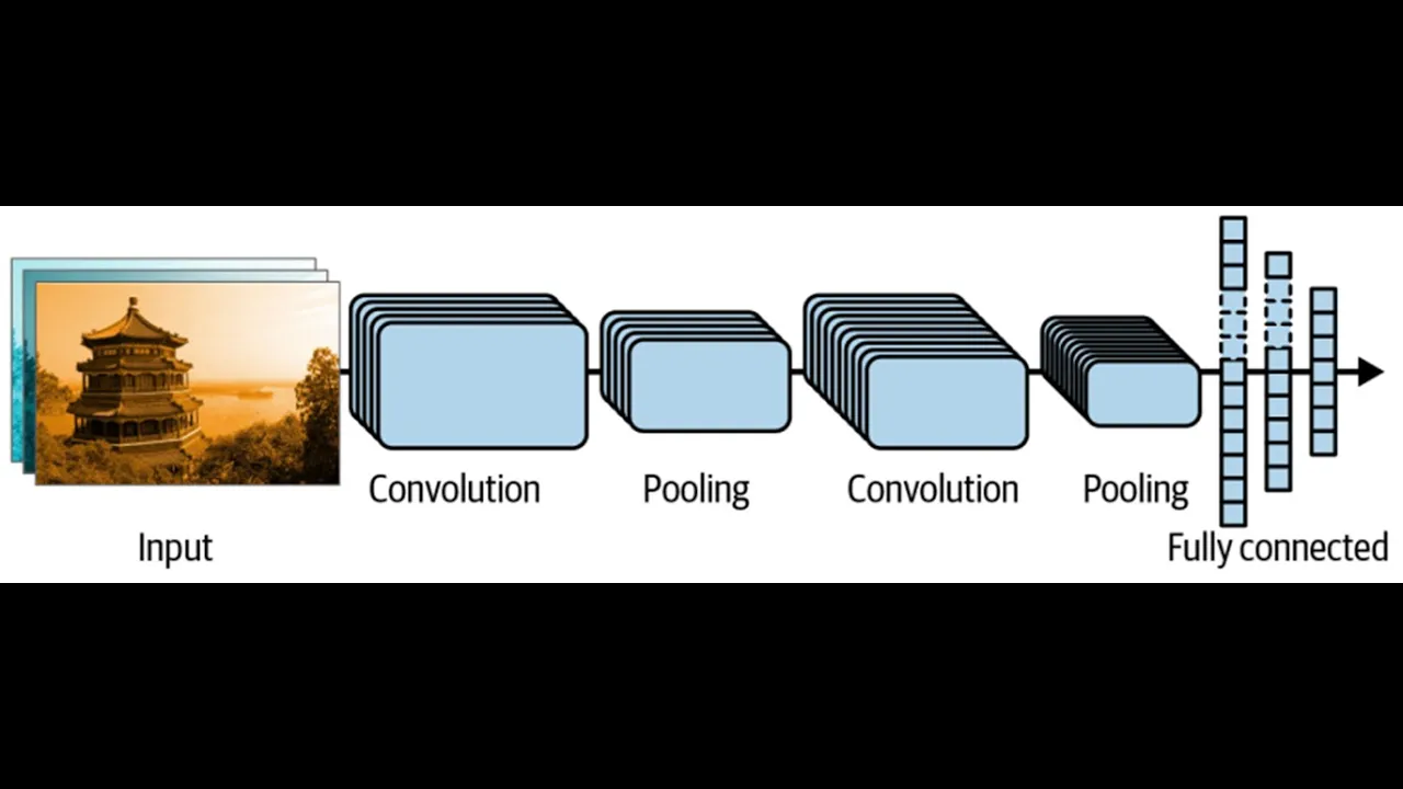
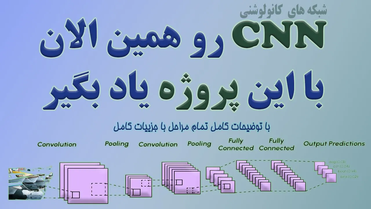
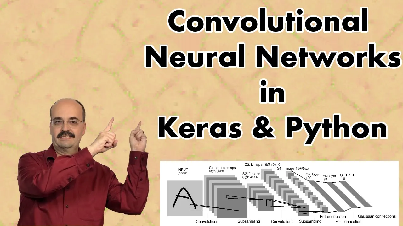
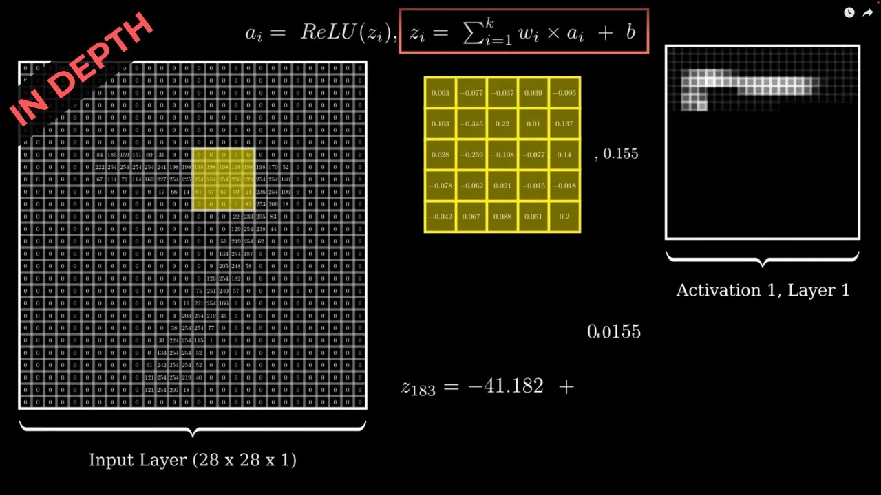


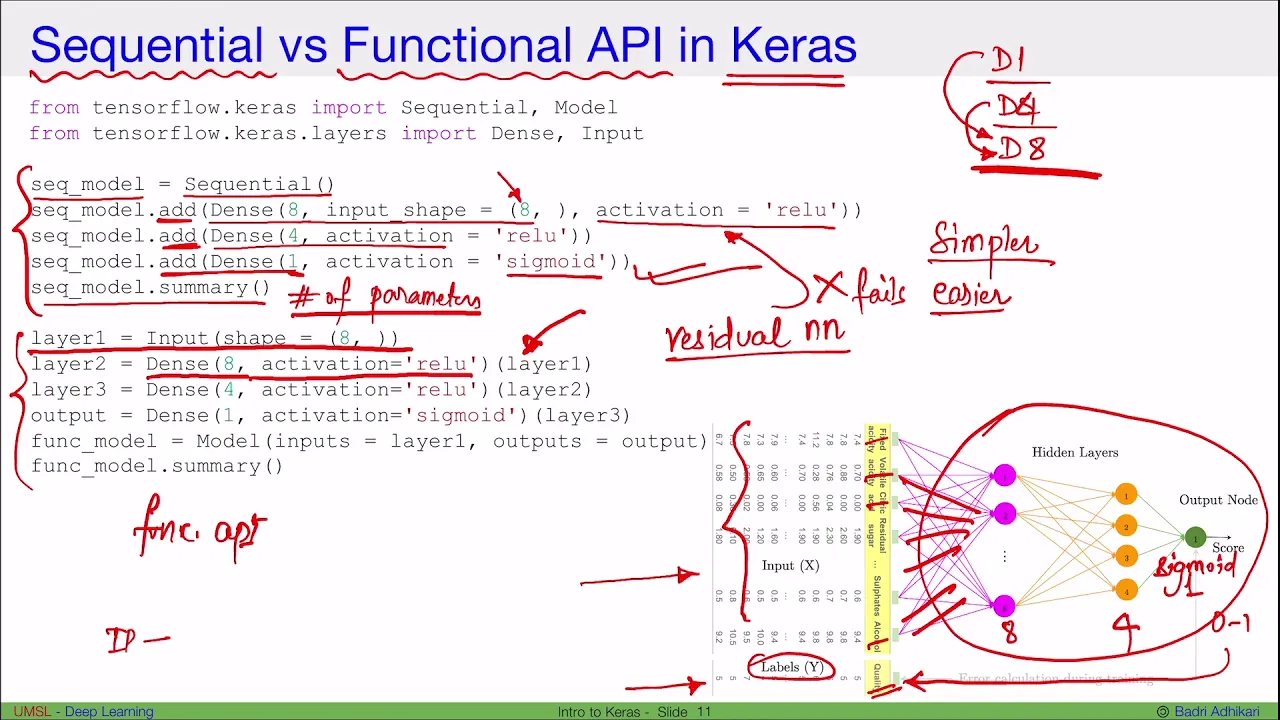






TensorFlow 2.0 is Google's most popular deep learning library that works in three parts: data preprocessing, model building, and training/evaluation. It takes input as multi-dimensional arrays called tensors. The key improvements in TensorFlow 2.0 include cleaner APIs, eager execution for Pythonic code, and Keras integration at the core, which improves productivity and execution speed. The tutorial demonstrates building a neural network model using the Sequential API with Flatten, Dense, and output layers, compiling with loss function (sparse categorical cross-entropy), optimizer (Adam), and metrics (accuracy), then training and evaluating on the Fashion MNIST dataset to achieve approximately 88% test accuracy.
TensorFlow 2.0 Tutorial: Getting Started with Keras for Deep Learning
Added:Proficiency in basic Python programming, including data structures, functions, and object-oriented concepts.
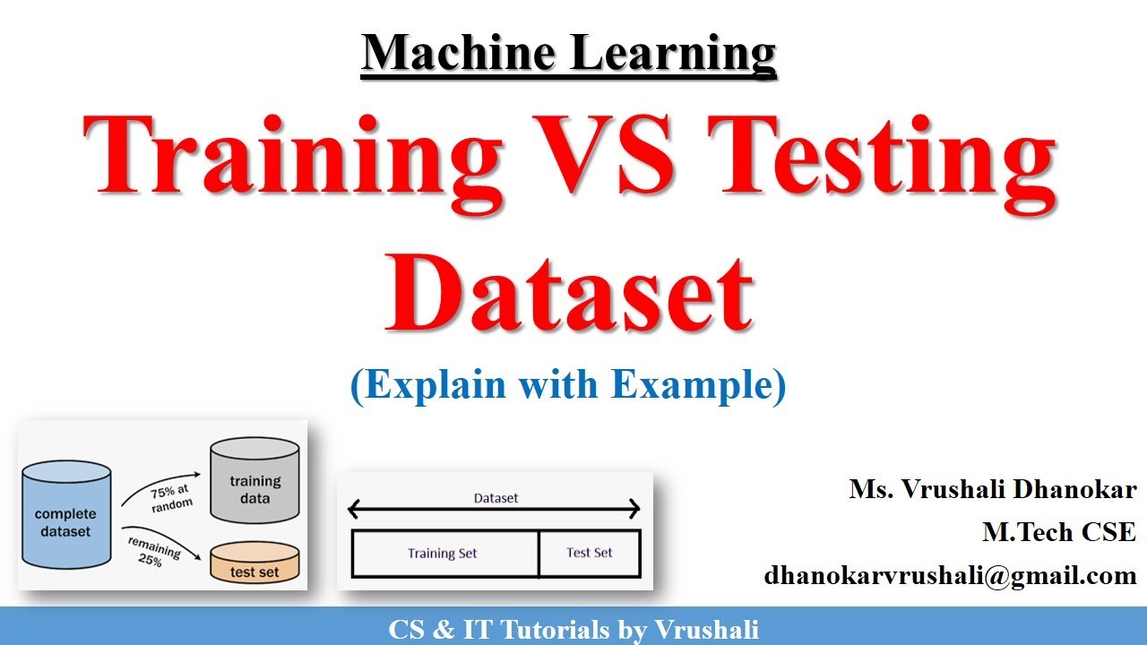
Fundamental understanding of Machine Learning concepts, such as supervised learning, training vs. testing datasets, and basic evaluation metrics like accuracy.
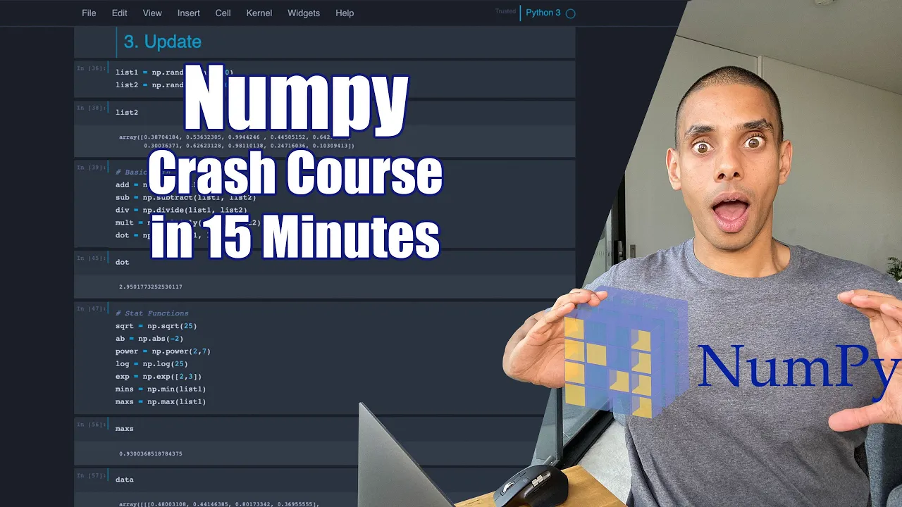
Familiarity with the NumPy library for data manipulation and working with multi-dimensional arrays (tensors).
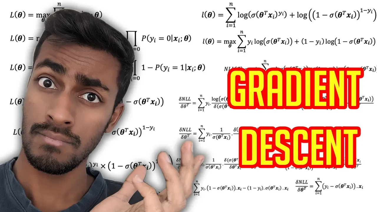
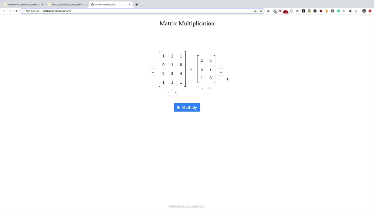
Basic knowledge of mathematics for deep learning, specifically matrix multiplication (linear algebra) and the concept of gradient descent (calculus).
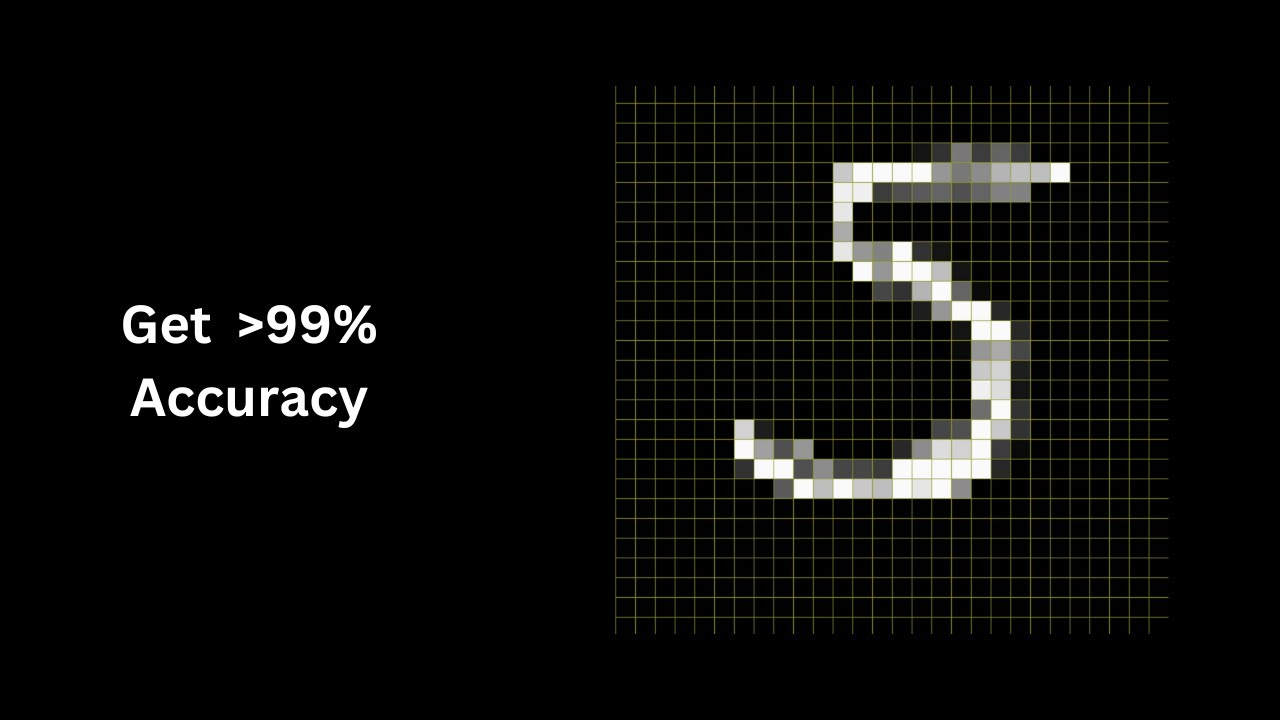
Exploring Convolutional Neural Networks (CNNs) to achieve significantly higher accuracy on image datasets like Fashion MNIST.
Mastering hyperparameter tuning and regularization techniques, such as Dropout, Batch Normalization, and L1/L2 regularization to prevent overfitting.
Transitioning from the Keras Sequential API to the Functional API and Model Subclassing for building complex, non-linear network topologies.
Learning model deployment workflows, including saving models, loading them for inference, and using TensorFlow Serving or TensorFlow Lite.
58.2K views562likes38:53Original Release: 2019-08-28
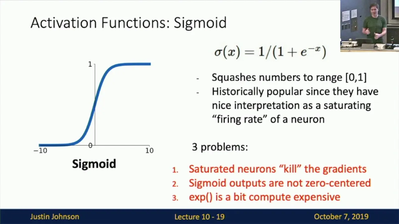
hi this is let's make antibody in this lesson I'm gonna start a very new video series on a deep learning so in the very first lesson I'm gonna start a deep learning with the tensorflow 2.0 okay so the tensorflow 2.0 - recently had it has been launched by the google and the google has promised so many you know and so many advantage of a tensorflow 2.0 over a tensorflow one point X so this we will be learning initially we will be learning just the introduction of tensorflow and how and why we should huge tensorflow 2.0 and then we will be working with the amnesty data set throughout this tutorial and then i'll show you how you can import the image dataset and then after that I'll show you how you can do some data exploration and after that I'll show you how you can build a model with tensorflow 2.0 and the Charis with the high level API and then finally how you can compile and then how you can train your model the maximum testing accuracy is training accuracy is 91% and the testing accuracy is 88% which shows that the model is overfitting somehow okay so this will be the all in this lesson before I start this lesson I would like to tell you one more thing you can go ahead at my channel kgp talkie and at the KGB talkie I have met so many videos I have basically made on the three basic topics the first topic was Python getting started so there I have covered the pandas numpy matplotlib Seabourn data visualization and then the second part of the lessons was on a classical machine learning like linear regression logistic regression K and in SVM decision tree random forest PC in symbol learning etc and the learning curve and then the third was based on a feature selection so I have selected the feature based on the filter methods wrapper methods and embedded methods as well as with the linear discriminate analysis and principal component analysis okay now come back to this lesson without wasting a time let's go ahead and start a brand you listen on a tensorflow 2.0 since this is a very sort and quick listen on a tensorflow 2.0 so angrily I'm gonna take a very quickly at through the part then I'll start a coating on this so once we start on the tensorflow the first come in our mind what is the tensor flow right so the currently the tensor flow is the most famous deep learning library in the world and Creech developed via Google the Google product uses machine learning in all of its product to improve the search engine translation image captionings recommendations moreover the Google do all these things to improve the user experience right so this tensor flow architecture works in the three parts the first it pre-process the data then it build the model and then finally train and estimate the models that's mean it train the model and then evaluate the performance of the model right and it is called the tensor flow because it takes input as a multi-dimensional array which is also known as a tensor that's why it is known as a tensor flow now the very quickly let's go ahead why every data scientist learns tensor flow to point X the currently the Google has released the tensor flow 2.0 the RC version which is the release candidate and why we should leave it in the flow one point X there are so many things which Google had changed into a tensor flow 2.0 okay so the tensor flow 2.0 make the users more productive including the are removing the redundant API and making API a more consistent the tensor flow one point X has many api's and the most of them were threatened dn't and the more I and the many times users get confused the data scientists get confused which is the best way and how to use those api's to get the better accuracy that means we had some let us say the particular task and for that particular task there were so many api's and the data scientists we're getting confused which API will be the best for their the data and for their model so in the tensorflow 2.0 the google has the deprecated and removed all those all those api's so the more overt google has done the api cleaner and it has uses the eager execution which is a pythonic breast moreover and it improves the execution time and while defining the variables now in the tensorflow 2.0 it doesn't Eugene into global variables and the tensorflow 2.0 has also removed this essence the earlier in tensorflow we had to use the system dot run and now the tensorflow 2.0 is kindly kind of bringing it like a function call and moreover now the tensor flew to point X R to find zero brings the clearance at the core of the tensor flow which ultimately increases the you know improves the accuracy that that actually can increase the accuracy but that is not 100% sure that that increases the accuracy but moreover it reduced the training and the testing time since the Kira's has been integrated with the core of the tensor flow and in that case the its execution will be the faster actually and it also takes a less space and moreover it is the consistent and if you want to know more about the tensor flow 2.0 what I it is offering you can go ahead and visit this link it has Google IO link there and at the Google i/o you can you know to see this the complete the getting started with the tensor flow 2.0 at the Google i/o so the air google has released this tensor flow 2.0 and they have covered almost everything what is the new in the tensor flow 2.0 there are so many things to the new into the tensorflow 2.0 although this is the new video series and we will be learning a lot about the tensorflow 2.0 throughout this video series now the let's go ahead the very quickly and I'm assuming that you have already installed the an akuna at the necessary library only you need to install the tensorflow and if you do remember the previously you need to install the chaos and the tensorflow separately but here you only need to install that cancer flow you actually don't need to install the Kiera's so you can call the pip install tensorflow equal to equal to the 2.0 RC and you can go ahead to this github link where you can get the tensorflow the released okay so here we have a tensorflow 2.0 and you can visit that I think with this yes so here we have a you know the latest tensorflow the 2.0 this this one is the not the latest one although with the website if you go and visit on the website there you will get a latest one the tensorflow 2.0 the release candidate is available and you just go ahead there you will get the link here to install this so you can keep monitoring this mission this link to get the updated version by the time I'm making this video this is the latest version now let's go ahead and open anaconda into administrator mode remember you need to open it into the administrator mode otherwise it would not be able to install the tensorflow 2.0 in your computer because of the right permission now let's go ahead and copy this which I can just copy it and in the anaconda right the pressing the right click it will paste here the PIP installed tensorflow equal to equal to two point zero point zero RC 0 that if the release candidate 0 let's go ahead and hit the enter although I have already installed the tensorflow 2.0 that's why it is saying that the all the requirement has been already satisfied but if you do not have the tensorflow 2.0 installed in your computer you can install and the moreover if you get the any error then you can first uninstall the previous tensorflow for that you can right there pip uninstalled tensorflow so it will uninstall your previous versions and then you can install a new version of a tensorflow okay perfect now let's go ahead and see if you have a GPU in your computer then you can also install a GPU version of a tensorflow right so these are the two ways where you can install a tensorflow in your computer now you can pause the video and pause this video and that you can continue this video after installing the tensorflow 2.0 alright now let's go ahead import the fashion mms data set so in this lesson we will be working on the finest fashion m-miss data set the fashion m needs to data set the link is available here and this working we working file is available in the video description from where you can download and if you visit this fashion m niche then you see here on the github the link is available and on the github it says that this is Jolanda article images it has 60 thousands examples and every sample have 20 28 cross 28 grayscale images and so these are the images and it has a 10 actually it has two total the ten classes and that's mean there are 10 type of the the fashion images are of level in this fashion amidst dataset okay so these are the images which are available and and and and this sixty thousand images which we will be using to train and ten thousand images to we'll be using to evaluate and it has total the ten categories of these images ok now let's go ahead and first import our learner now first let's go ahead and import the tensorflow and then I'll show you how you can download this the amnesty data set directly into your Jupiters notebook instead of downloading it from a geek health ok / pets to import the tensorflow you need to write their the import and then the tensorflow there we have a tensor flow as usual tensor flow as DF and then we need to improve the care as from the tensor flow so here we have a from tensor flow import the Kira's okay so now we have got sorry we have got the tensor flow and in the chaos sorry yeah now we have imported the Kira's from a tensor flow now let's go ahead and import other necessary libraries like numpy pandas and the matplotlib so those things we can say that a helper liability but before that let's go ahead and check a tensor flow version which you can just check from a print T F dot version so this says that we have Overson 2.0 installed in my computer now let's go ahead and import helper libraries like an umpire Pentagon the matplotlib so in the previous videos we have been importing these libraries very frequently numpy as in P and import pandas HPD and then import might float lib dot type lot as PLT so here we have matplotlib i the pandas and the numpy imported in our computer so these things we can treat as a helper libraries now let's go ahead and load the amnesty person dataset so for that i can write here the amidst is equal to the Kyra's dot datasets and then I can write there the fashion I'm honest so with this we will get a pass anemones dataset although I have already downloaded it my computer otherwise it might take a little time in your computer to download this data set from a internet that might take a few seconds if you have a fast internet now let's go ahead and check the type of the immunised this says that with this immunised actually it has downloaded the data sets in a tensor flow module wrapper now what we need to do now we need to actually load the data now we need to load this data into into a real real variables in this jupiter notebook and to do that it actually returns a tuple ok the two tuples wonderful for the training and another tougher for the testing so for this what we can do here the m in each dot a load data set as usual we have been doing into a scalar now in this topple we need to first down get the data into our our the training dataset that is the extreme and then finally Whiterun and the next couple in the next it returns the testing data sets it has X underscore test and then Y underscore test so it has a 60,000 rows for a training which we can verify that with X train dot safe now there you see here there are 60,000 images are available there and each images have 28 cross 28 some since there are 60,000 images that's mean it should have a 60,000 y train as well so let's go ahead and check the safe of Y trend which says that it has a 60,000 okay now let's go ahead and print the X train and see what happens once we print the extreme we see the values the most of the values we are printing here 0 that is because you note at the ages since this is the grayscale so at the edges the most of the images values are 0 otherwise the maximum value inside this the area which we can find that within P dot max okay so that's it the 255 so the minimum we have already seen in there and that that is the zero but here are the max is 255 and if we see the average that's mean the N P dot mean the X train so it says that something so moreover now we can we can say that the values is somewhere in between 0 and the 255 okay inside this data set which we later we need to bring down in between 0 and 1 to train with the tensor flow tensor flow model okay our deep learning model and these 60,000 images are classified into ten labels and those labels are encoded into a numerical values and those numerical values we can see with the Y under escort rain and those numerical values are in between 0 & 1 sorry 0 1 9 okay so it starts from the 0 until the 9 so those are the 10 categories there now let's go ahead and write those category names although you can get on the pass and M minister's category names there you should get those category names somewhere here yes which category names are here okay so these are the desert trouser pullover dress code sandal cert sneaker back at the ankle board now let's go ahead and and write that the class names here so that we can write in new variable the class name and inside those class name we need to write it okay the desert sign the topic cetera like here we have let us go at the top and the Ender when we have here at rapture and then here we have the pullover and then here we have dress then we have a court and then finally we have the sandal and then we have a cert and then we have a sneaker and then after that we have back sorry it's bad actually not a bad and then we have ankle boot so these are dipped in classes right now let's go ahead and do some the the data exploration so with this data exploration we can actually understand our data in in more explode way okay so since we already have seen its you know the same etc so here if we see the X underscore the train dot say we have 60,000 images but if we see here X underscore test dot safe there we see we have just 10,000 images so this 60,000 images is available for a training and these 10,000 images available for testing purpose so that we can test our model and we can see how accurate our model is performing now let us go ahead and visualize the visualize the data some images so we can visualize that with the PLT so here we have a PLT door failure and then we have a PLT dot image so that's the I am so and inside that we are gonna the see first image okay that is the extreme zero and then I'm gonna just see it and now you will see here it has this image okay so this is actually the boot okay and how would you know this is boot and if we if we print here the X screen actually there you see its nine number and at the nine number you see here we have ankle boot okay so this is the word and if we see here one number and now you see had the one number it's a zero and at the zero it is at top okay so this is how we can visualize and if we print here a color bar at the side okay so we can just right there the color bar okay so with the color bar now you see we have here a color bar and this color bar now you see the value is somewhere in between 0 and the 255 since since neural network model doesn't take the value greater than the one that's mean we need to bring down this the value in the maximum value the 255 in between somewhere 0 and 1 so what we can do to bring it down we can just divide the value with 255 I mean the training and the testing data set with the 255 so we can get here with X underscore X underscore train dot sorry X underscore train is equal to X underscore sorry X underscore train and then divide it by two fifty five point zero okay perfect all right so we have got the extreme in between 0 and the 1 and similarly let's go ahead and bring the X test in between 0 & 1 which we can get by dividing X test by 255 point 0 so with this we have got our X train and the X test in between and in in between the 0 to 25 and what we can do we can just copy it although you need to use your keyboard control and the C and let's go ahead and paste it here and see what happens now now with this you can see here we have brought it down in between 0 and one okay so now this this value is now ready to feed into into into a neural network and one more thing you might have noticed that this size it's a size is 28 cross 28 that's mean there are 28 pixels and these are the pixels which you can see okay so these are the pixels a square dot there so these are the 28 dots here and the 28 is here okay perfect now let's go ahead now build a model a machine learning model with the tensorflow 2.0 with the f 2.0 okay so so so in this what we are going to do the basic building blocks in any neural network is a neural network layers okay so the lyric extracts the representation from the data and Anthony peered into into into it's a hidden layer actually and then finally it starts the training okay so although this is the very critical instance on the tensorflow 2.0 and I'm assuming that you know a little about the neural network so basically you understand how the neural network works so let's go ahead and import the sequential and the dense model sequential and the dense layers from tensorflow Kira's to do that what we can do the front ends are flow from the tensorflow dot Kira's import sequential and then from tensorflow dot dot Kira's and then got layers import and from here I'm gonna import the flatten layer that will be used as a first layer and then dense layer so we have got the two layer and flatten and the dense and the sequential model now let's go ahead and create our model so here we are gonna build our model with the sequential model so here we have a sequence here and then we are gonna pass here ready okay so so the area means the how many are the layers we need inside our sequential model there are many ways to build this but I think this is the simplest way where we can add all these together otherwise there are a few other ways like like just defining first sequential and then going with the model dot add we can go ahead with that one as well like model dot add and then we can add there the first flatten layer there and inside the flatten layer the input shape okay which we are gonna use here input shape will be the 28 cross a 28 there okay so this is an input safe for our the flatten layer the flat hair doesn't do anything actually it's just transformed the the formats of this data which is 28 cross to 28 so this this layer just transformed this data into a one dimensional so that we can fit into the next layer okay so the next layer which I'm gonna add here in the model dot and that is a dense layer okay so this is just a dense layer and inside the dense layer if you press your sift and double tab you will get here detail the documentation on it so in this I'm gonna pass the number of units that's been the number of nodes how many the neural neurons actually we want and then we will pass here the activation function which activation function we are gonna use I'll be taking a different lessons where I will be covering all these things in a very detail this is a very quick lesson so I'm not going to cover all those things here in the detail so activations we will be using and other things we will be just passing as usual okay so other things will be like yeah other things will be a default actually so here in the dense layer I am gonna pass here the 128 new rooms at the firstly and the activation function which we had talked there that I'm gonna use here a raloo activation so this is kind of the detective higher the activation function there are so many other kind of activation function like a sigmoid an edge and you know the Rayleigh key relive all those so here for this listen I'm just gonna use your a loop and then the model dot ad and then again I'm gonna use the output layer in an output layer if you add the output layer then we need to define the how many outputs are there that's when the total number of classes we have a ten classes that's when we have to define here the ten and the activation function here so at the output the real you activation things an activation cannot be used so there at the output either we can use the sigmoid or softmax so here we are gonna use a soft max okay so here we have a model now let's go ahead and print the summary on this model and then you might understand how it is building so the first model has transformed a two-dimensional data into a single dimensional and then here we have 128-bit 128 neurons so 128 and then multiplied by that 784 its complexity reaches the number of parameters actually then reaches to these digits okay so that is the hundred thousands and then finally at the output we are bringing it down to the ten okay jester ten so we have number of parameters at the final output to calculate it the twelve hundred and ninety okay so the total parameter which we which this model will be executing is more than 100,000 okay so this is how we build the model now we need to compile our model okay so for compliation of the model there are a few things which are really very important okay the first which need we need to actually define sorry we need to convert it into a markdown yes so the first thing which we need to define is a loss function okay model compliation so to compile the model we need to define the loss function which loss function we want here and then we want optimizer okay and then after optimizer we want here metrics so what are these things a loss function it will measure how accurate the model is during the training and testing then okay actually the loss function minimize minimize the overall error during the training and once the error is minimized during the training then the testing error will be also minimized but that is not always the true because sometimes what happens if your model overpaid then the oral law skit minimized during the training but during the testing it get increased so here the generalization of model is very important that's where optimizer comes so this is how model is updated based on the data that's been the weights of our model applicants updated with the you know as we define the optimizer now let's go ahead and compile this model first so we can compile this with the model dot dot the compiled and then here we have optimizer is equal to Adam and then here we have a loss function there a loss is equal to a spazz categorical okay so there we have a sparse and categorical cross entropy okay and then finally here we have a matrix and inside this matrix we have accuracy okay perfect now let's go ahead and run this and once we run these Suites its of course it's it has compiled there now let's go ahead and train the model for a training a model it is really very simple as we have been doing into our SQL library there we have a mortal dot paid and then here we have X underscore train and then here we have y underscore train and then finally here we have a total number of epochs okay is equal to 10 so with this once we write this it will start suing a progress bar our during the training so the first time at the first epoch itself the accuracy has increased to 82 now do you know the epoch the epoch means at the first time the you know the weights get initialized randomly and when model moves to the second day pork then via back propagation it updates the model that's mean what it is doing at the ten times it is updating the models and then it is running on whole data and each epoch okay that's minify defining your a box is equal to the ten then that so in this model this this model is getting trained ten times on whole data that's mean the weights are getting updated ten times on the whole data now let's go ahead and finally evaluate the accuracy of the model how we can evaluate the accuracy to evaluate the accuracy and the tensorflow has inbuilt model dot he will wait but in this video version that is not working very precisely that's me let's say if I write here a test loss and then the test accuracy is equal to model dot evaluate okay so there it has X underscore test and then Y underscore test okay and then if we print here the test I Chrissy let's go ahead and see how much this tie Chrissy we will get here so this this is a kind of there is a problem I think perhaps that's why it is you know suing these random things although this will take us some time just around return 10 to 20 seconds and then it gets completed and then finally it will the source total accuracy on a test set okay now you see here the tests accuracy on test set has been shown at the end of this that says that the eighty eight point seven five percent of the accuracy Rd test and the total loss is zero point two five now you see here during the training our accuracy was a 91% and at the testing time accuracy is 88% that shows that the overfitting of our model so this is kind of a very simple neural network model just similarly just a single layer is there just a single hidden layer with the 128 neurons so we can expect that this much of the accuracy with this although if we use Union and other networks on this then we definitely we can get a better accuracy okay and on the github it it is claimed that with the CNN we can get around to 99% accuracy in some other lessons we will be also learning it with the CNN as well now let's go ahead and do the prediction with the now let's go ahead and do the prediction with the with the Escalon as well okay so what we can do here with from s killer dot matrix and then here we have import a crazy score okay so now we are we have here we have here accuracy sorry now we need to first get the wipe read as well so that we can get here Y prayer is equal to the wipe rate is equal to the model dot predict okay now you see here we have the two classes actually the predict and the predict classes and the predict probability so the predict will predict a set of the array that will be the continuous value but we need a predict classes so with the predict classes we can get actually what is the predicted class instead of a continuous value on yesterday doesn't that is expressed and then finally let's go ahead and bring it with the accuracy score that here we have y underscore test and then here we have y underscore bread so now you see we have got the accuracy of eighty eight point seven five percent which we have caught with thee with the model dot evaluate although I think there is some bug in this current version of the tensorflow that's why these things we are coming okay perfect now let's go ahead and make a prediction on adjust to some random the random test the image on us just a single image separately and then we will stop this lesson okay to do that what we can do you can just right there let's go ahead with the bread played with the model dot a simple predict and then finally we have here X underscore test now if we print here the bread so the prettiest kind of you know a continuous array that's why I had not done with the predict only that's why I had used here the predict classes and if you see there the wipe read the wipe read here is continuous its its categorical value actually that's been the classes okay so with this now let's go ahead one thing you see and the class has been predicted the first class has been predicted to nine and if you see here the first array the continuous value now you see here at the ninth one okay that's in the tenth class tenth number at the ninth index at the tenth index that's mean you know zero it starts from the zero that's been here nine so it says that at the 98th sent with the confidence of the 98% that it is the ninth okay what we can do now we can prayed here at the zero value now with this you can we see it very clearly okay so this is the maximum out you know the ninth place so that how we can do we can do with the org max here okay so here we have n P dot arcamax there's been the maximum argument at which place there so that's the Preds ero at the plate 0 you see maximum argument at 0th location and similarly we can bring this the maximum prediction at at the first location as well okay so at the first location the maximum is you know the argument - okay perfect so this is the way how we work with the tensorflow 2.0 this is all about in this lesson please don't forget to like this video and subscribe this channel so that you can get updates directly into your inbox in further lessons all week also covering more videos on a tensorflow and deep learning till then bye bye and keep learning
Up Next

8:36
Content-Based vs Collaborative Filtering for Recommendation Systems
@TensorFlow
89.1K views•2021-07-06
87:26
Introduction to Secure Multiparty Computation with Yehuda Lindell
@fhe_org
7.7K views•2021-02-04

4:55
HTTP Requests Explained: GET, POST, PUT, DELETE
@codecademy
103.1K views•2021-10-07

19:25
Enigma Machine Mechanics: WWII Encryption Explained
@JaredOwen
13.2M views•2021-12-11
Related Study Plans & Knowledge Roadmaps
Structured learning paths in Computer Science
computer-science
Container Runtimes: Namespaces, Cgroups & Go
01Linux Systems & Go Programming Foundations
02The Core of Isolation: Chroot and Filesystems
03Linux Namespaces: Process Isolation
+ 3 more learning modules
32h6 modules
Explore Roadmap
computer-science
Building a CHIP-8 Emulator: Rust & CPU Basics
01Computer Architecture Foundations (Bits & Bytes)
02Rust Programming for Systems Development
03CHIP-8 Virtual Hardware Specifications
+ 2 more learning modules
32h5 modules
Explore Roadmap
computer-science
Building BitTorrent: Go, P2P & Concurrency
01Go Fundamentals & Concurrency
02Networking Foundations & P2P Architecture
03Bencode Parsing & Torrent Metadata
+ 3 more learning modules
26h6 modules
Explore Roadmap
computer-science
Actor Models (C++ Concurrency & Lock-Free)
01C++ Multi-Threading Foundations
02Thread Pools and Task Scheduling
03Atomics and Lock-Free Queue Design
+ 3 more learning modules
45h6 modules
Explore Roadmap