






![[TUTORIAL] PYTHON para Análise de Dados - Aprenda do ZERO](https://i.ytimg.com/vi/FZODEbfcDwU/maxresdefault.jpg)
![Как анализировать данные с Python библиотеками Pandas и Numpy [GeekBrains]](https://i.ytimg.com/vi_webp/lLf6Qt6wSJ8/maxresdefault.webp)











![[Visual Python 2025 Machine Learning] #06. 앙상블 - Random Forest XGBoost LightGBM | 비주얼 파이썬](https://i.ytimg.com/vi_webp/MiaSdqDE40o/maxresdefault.webp)
Classification is a machine learning technique for predicting categorical labels (like good/bad wine) rather than numerical values, and unlike accuracy, proper evaluation requires using confusion matrices, precision (TP/(TP+FP)), recall (TP/(TP+FN)), and F1 score (harmonic mean of precision and recall), along with ROC curves and AUC metrics, because accuracy alone can be misleading in imbalanced datasets; the implementation involves preprocessing data, splitting into training/test sets, scaling features, training classifiers like SVM or Random Forest, and tuning hyperparameters using grid search to optimize performance.
Hands-On Machine Learning: Classification Algorithms Explained
Added:Basic Python programming proficiency, including familiarity with variables, functions, and standard data structures.
Fundamental concepts of supervised learning, specifically the distinction between features (inputs) and labels (outputs).
Basic data manipulation and analysis skills using Python libraries such as NumPy and Pandas.
Introductory knowledge of statistics and probability, particularly concepts like ratios, percentages, and conditional probability.
Advanced evaluation metrics and diagnostic tools, such as the Receiver Operating Characteristic (ROC) curve and Area Under the Curve (AUC).
Strategies for handling highly imbalanced datasets, including resampling techniques (SMOTE) and cost-sensitive learning.
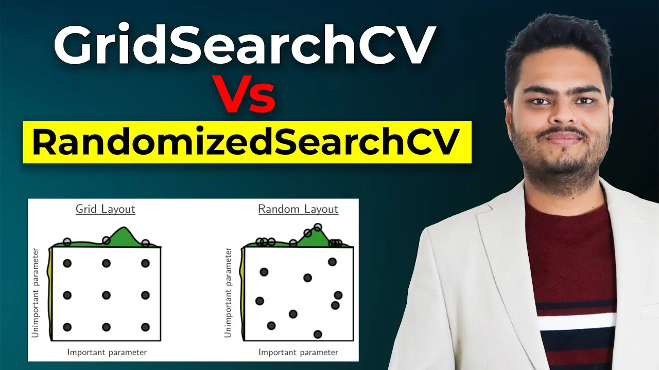
Hyperparameter optimization and model selection techniques using Cross-Validation, GridSearchCV, and RandomizedSearchCV.
Ensemble learning methods for classification, such as Random Forests, Gradient Boosting (XGBoost), and stacking classifiers.
25.1K views551likes47:14Original Release: 2021-05-09
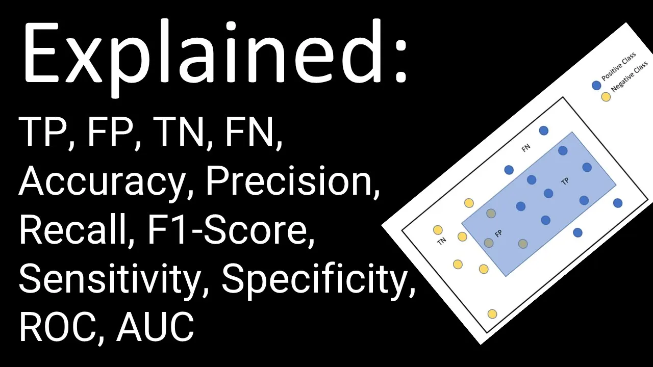
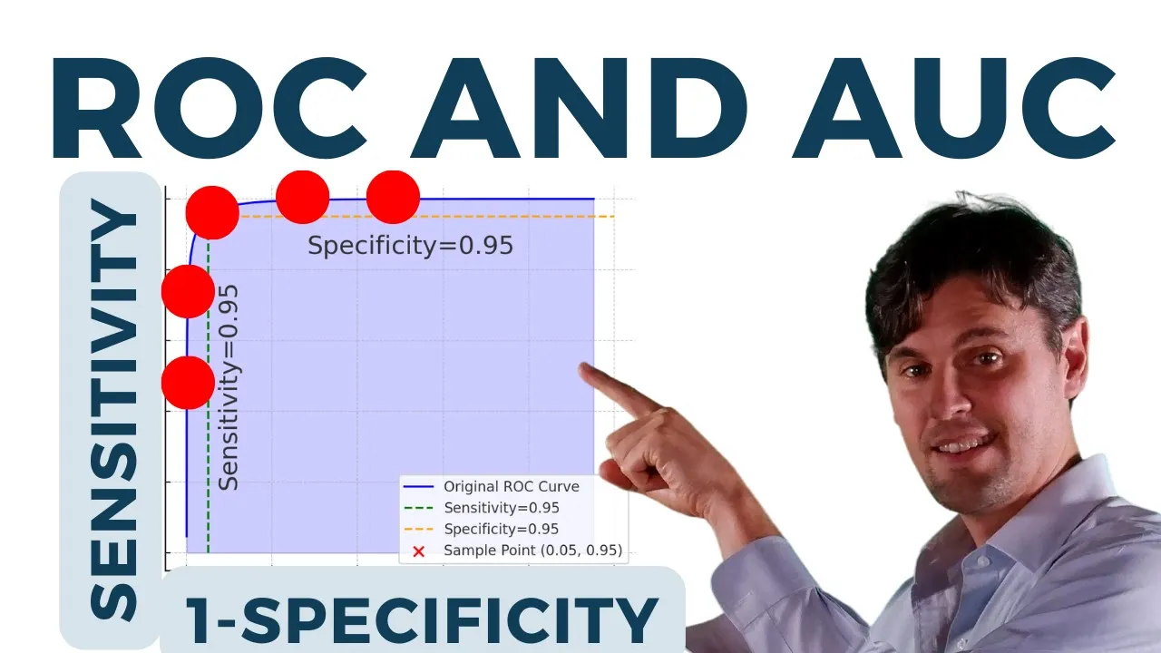
shashankalanithi and today we're going to be going over hands-on machine learning with scikit-learn karos and tensorflow um a book by aurelion garone this book is considered by many to be kind of like the de facto handbook for machine learning this is where you get started if you want to learn uh which is exactly what i'm doing right now i'm a data analyst and i'm looking to become a data scientist in the future and you know i would like to learn how machine learning works at a deeper level than you know uh some tutorials online would uh would take you um so if you're going through this journey with me you'll know that chapter two we put that video out last week where we went through an entire machine learning project from start to finish and we're doing classification today which is chapter three of the book so what is classification versus regression so basically when it comes to machine learning algorithms you have many different problems that you can solve the two biggest ones are probably um where you have classification and regression and with regression you basically have a regression is when you're trying to predict values so for example if you're trying to predict the revenue that your company will have next year that is a regression problem when you're trying to predict the quality of wine as in good or bad that is a classification problem so today we'll be working on classification problems all right so before i get started i do want to let you guys know i do have a patreon and all these notes and the code that i'll be writing will be available over there it is a great way to support me and my work i put out videos i try and put out a video about once a week of just you know stuff i'm doing as a data analyst and the um anything that i learn uh over the course of you know my studies um in the world of data data analysis and data science um so if you feel that my work is worth supporting or you would like to have access to these notes which i do constantly update then please let me know and uh let's get right into it so with classification in this chapter he spent a lot of time talking about performance analysis and the reason for that is because with classification algorithms unlike uh regression algorithms performance analysis can be a little bit more difficult because accuracy by itself is not necessarily a great measure of how good a classification algorithm is and a great example of this is for example if you're trying to predict um out of a thousand people how many people have cancer let's just say cancer has a less than 99 or has a one percent um uh incident rate amongst the population right if your algorithm just says no one in a population has cancer at all it is a 99 accurate algorithm but it's not quite what we're looking for here so that's why we spend we're going to spend some time talking about performance measures how do we measure the performance of our algorithm before we actually get started with uh writing our code for it so the first thing that you're going to want to do is you're going to want to create something called a confusion matrix and all a confusion matrix is is that it's a matrix that compares every prediction your classifier makes with the true value of that prediction so what do what is that what do i mean by that it'll come out in a um x by x grid um x being the number of classifications that you're outputting so we're using a we're making a binary classifier here meaning that we're predicting yes or no to something and uh you know binary there's only two choices so when you get an outputted when you get a confusion matrix output output by your algorithm like this the predicted values will be on the x-axis and the actual values will be on the y-axis and what does that mean that means that for example over here 1 means positive or true and then 0 means negative or false so that means if you predicted one and the actual was one it'll show up over here and that is a true positive if you predicted zero negative and the actual was zero which is negative then the value will show up over here you want most of your values showing up on this main diagonal over here you know goes up and down like this the main diagonal and you'll see over here with this algorithm you know that i created earlier that is exactly what's happening it is going um the main diagonal is has the majority of our values so this is you know a decent predictor at least what everything else is going to be your false positives and your false negatives basically where you predicted a positive but it was actually a negative so you see we predicted positive one but the actual value was negative or we predicted negative and the actual value is positive that's a false negative so we want to avoid those so now we've created a confusion matrix and you know all the confusion matrix is basically you take every prediction that you make and you just put it into whatever bucket it belongs to you can start running some uh equations to get precision and recall or sensitivity and an f1 score and these are basically alternative ways to measure the accuracy of your algorithm so for example precision is basically a measure of how often your positive end predictions are actually accurate now what does that mean you'll see over here the the formula is true positive divided by true positive plus false positive so let's uh let's actually illustrate with an example so you'll see over here let us make this a little bit smaller okay so we have our confusion matrix over here um let's do one more thing there we go awesome okay so we have our confusion matrix over here and as you can see we've predicted positive a true positive 789 times we've predicted a true negative 200 times a false positive once and a false positive i mean a false negative 10 times um let me go ahead and make this a 51 and then remove 50 predictions from here so 7 39 and that i believe should still leave me with 1 000 yep 1000 awesome so if we wanted to so first of all let us go ahead and um let us go ahead and classify everything as either true positive false positive true negative or false negative so i'm going to color these over here oh well i like true positive so we'll make those green we'll make this also darker shade of green true positive true negative and then false positive and false negative so you can see what we have over here the true positive is cell d4 which is this over here false positive is right over here d3 c4 is a false negative and a true negative is c3 so using that we can calculate our precision so what is precision precision will be b6 which is what over here true positive divided by true positive plus false positive 51. so what is that telling us that's telling us that every time every time our classifier predicts a positive value it's only accurate about 93 of the time you know i mean you know obviously this is a good classifier but like um that would be different from uh accuracy for example i should also probably add accuracy here so let's uh we'll call this one accuracy and accuracy would be equals the true positive plus the false positive divided by everything else so it's a very subtle difference over here but you can see that um you know if i was to like skew the values a little bit more it would change a bit so like you know we're seeing accuracy is at uh 0.939 but precision is only at 0.935 um which is basically telling us that we're uh mispredicting some of our positive values we're saying things are positive but they're not actually positive um recall and sensitivity is basically the true positive so 739 divided by 739 which is again your true positive plus your false negative over here and then what happens is you can combine these into something called an f1 score um an f1 score is basically the harmonic mean which is just another way of calculating a mean versus um you know the normal way you'd use you calculate means um it is the harmonic harmonic mean of precision and recall and what this what a harmonic mean does that's different from your regular means is it more heavily biases lower values um and there's a little bit more written about it over here uh oh okay i should probably finish my notes over here but basically gives more accuracy to lower values and then what happens is you'll eventually run into something called the precision recall trade-off so how does a algorithm actually classify things into these different categories over here well what it does is it gives a probability to every single classification and then what happens is that probability or more than the probability gives a value to every single instance in your data set and then what happens is you can set a a threshold get set you know anything that's above this threshold call that class one anything that's below that call that class zero um and what happens is if you increase that threshold your algorithm becomes more and more strict basically meaning it's harder and harder for to classify things in the positive true class and if you don't do if you lower your threshold like things are more easily classified as uh as in an accurate manner so as you can see over here as you increase your threshold you are actually you can you will increase your precision naturally and you will decrease your recall at the same time but if you decrease your threshold you're creating a less precise algorithm but one that has greater recall so this is a chart that you'll become very familiar with and you can use to determine okay like what is the threshold we want to set our algorithm at what's more important is precision or recall depending on what you're looking into you may decide to pick one or the other and then i have the code over here which we're going to be executing on fairly soon another accuracy measure we're going to be using is called our the roc curve or the repair receiver operating characteristic curve and it's used for binary classifiers again when you're just classifying two different things um and it plot it plots the true positive rate which is recall against the false positive rate basically how many times did you predict something to be positive and it actually was positive versus how many times did you predict something to be positive but it was not positive um and then you'll see the calculation for the false positive rates over here basically it's one minus specificity and what happens is you plot the roc curve against the um uh curve of um i'm not exactly sure what this call but this curve is basically if you were to randomly guess so for example if you have a binary classifier the worst predictor you can have is one that would equally predict one class versus another you know it's basically randomly predicting um if you have anything worse than that it's worse than randomly guessing so you definitely don't want that so the amount that your curve is above this rand and this uh randomly picking line over here the better your algorithm is um and you can measure that mathematically using something called area under the curve auc so the area under the curve 0.5 it's a completely random classifier and if it's one then it's a perfect classifier so this is just another metric you can use so if we want to actually execute and run a classifier we can go ahead and get started over here um so i think i'm going to be using the wine classifier here yeah we'll be using our own classification task so we'll be bringing in the wine data set so and i'll make that available in the description below and this is basically a really famous data set that was created by the university of california and irvine they have a repository of data sets that are really popular that you can use for your machine learning tasks so we'll say data import equals pd.read underscore csv oh you know what let me write my boilerplate code first so all i'm doing over here is i am creating a uh the file path to the file that i want to get to i think it's called yes it's called wine so nothing special here all we did was we imported pandas you know the panel data library in python we defined our present working directory as the current directory that our that our file is in and then we said our file path is basically os.path.join which basically just combines two things in an os agnostic way um present working director directory plus wine dot csv um and the reason you want the to use this instead of what i used to do is because uh windows for example will use a double backslash um for its file pads and uh os 10 mac os we'll use a forward slash so that's why we want to use os.path.join it'll detect your operating system and then just create a file path that's accurate to your operating system all right data import okay so we have our data and as we can see over here quality on this side over here is what we're trying to predict so as you can see quality um and let me actually plot it out over here so data underscore import quality dot hist hist so as you can see our our wine qualities are rated anywhere from three to eight and so we're just gonna arbitrarily designate that anything um let's see above five so six seven eight is a good one and anything five and below is a bad wine and that's how we're going to create our classes because currently this is a little bit more like a well it's not it's not necessarily a regression problem but we're going to be creating a binary classifier so we're going to try and classify wines as either good or bad so this data set has a bunch of information on it you know how much acidity is inside the wine citric acid residual sugars chlorides um densities and there are actually like mathematical measures you can um use to determine okay like is this going to be a good wine or a bad wine there's some stuff that's just more popular in good wines versus bad wines so let's go ahead and do our classification test so first we have to create our classes so let us say um the first thing we need to do is split our data set into an x and a y data set x being what we're going to be using to classify and y being what we're actually classifying so y equals data import to our data import quality is greater than 5 and as you can see what that did is that basically creates a panda series of uh true or false true if the value is greater than five false if it's five or less um and discrete these are our classes right here it's as simple as that and then we're going to say x equals uh data underscore import dot i lock so basically in index loc i've got an llc stood for but index llc we want all of our rows so um remember the for these things too the normal format is basically your rows go over here which rows you want go over here where my cursor is right now and your the columns you want to include go over here where my cursor is right now so we want all of our rows so if i just hit a semicolon it'll automatically include all of our rows um if i wanted to only include rows one through three well there you go so if i do this it'll include all of our rows okay then let us in import uh we want all of our columns up until the last one and the reason you'll see is if you see here the last one is quality we don't want quality to predict quality because quality is a perfect predictor of quality so we need to drop this column and that's one way to do it and i'm just hitting uh shift return shift enter on windows to run the code so you can see we have all of our columns except for quality awesome okay so now we need to do a train test split basically we need to create our training data set and our testing data set um and what happens is we train our machine learning algorithm on the training data set and then we test it on the testing data set to see okay did you actually learn something and the reason we want to keep training and testing separate is because you want to make sure that you have some way to accurately test how your algorithm will work in the real world and that's by training it on certain data and then testing it on data it's never seen before which would be our test data set we're going to isolate that um you can ensure that your algorithm or you can predict how your algorithm will work in the real world so let's go ahead and let us do sklearn so from sk learn dot model selection there we go import train test split um and then usually the format for this is x train x test y and if you don't if you don't remember this don't worry i mean i've typed this code out so many times that you know of course i remember it now uh equals train test split and then we need to give it our x value so remember our x value is just this x we created over here our y value what we're trying to predict that's over here so x is what we're predicting with y is what we are actually predicting like a normal formula and then i want my test size to equal 0.2 and then i think random what is it random what state that's a yeah and all that does is that make sure that the uh for example if you run this code if you uh you should get the same train testbook that i get if you use random state equals 42 but normally you'd want to use a completely different number or you wouldn't want to include it at all and then let's inspect our x train set we don't want to look at our x test set at all cool so you'll see we went from 1599 rows to 1279 rows so our split worked okay so the good thing is we have no categorical variables in here um and i picked a dataset that had no categorical variables on purpose that way we could actually like um that we don't have to worry about like encoding those categorical variables the next thing we have to do is scale our variable so let's go ahead and do that so let's see from sk learn dot i think it's uh pre-processing import standard scalar and then we need to create our scalar object so basically that's just going to be scalar equals standard scalar and then we need to fit our scalar object onto our training set so we'll do scalar dot fit we'll fit transform because we also want to transform the data set uh x train i think i can do it like that okay no i have to actually say scaled and don't worry about this i'll explain in a second okay so what we did over here is we scaled our data so if you remember from chapter two um and if none of this sounds familiar make sure to watch my chapter two video that goes over we go over all this stuff um scaling a lot of machine learning algorithms especially stuff like linear models uh will not work well if for example one of your columns goes up to the value of a goes anywhere from 0 to 11 but the other values are only from 0 to 1.
basically it doesn't know how to reconcile those two like wildly different scales once 11 times the other one um and so what happens is when we scale our values we bring it all down to the same scale that way we don't confuse our algorithms many algorithms these days will actually do the scaling themselves um but i like to do this just to you know eliminate that potential for making errors so we what we did we brought in the standard scalar from the sklearn preprocessing library we created a scalar object so basically this variable scalar is a standard scalar object now and then what happens is we took our x training data and we told the scalar okay learn how to scale data based on this data that's called fitting when you fit two things together and then transforming is when we i said okay now that you've learned how to scale that data actually transform the data so what you could also do is you could actually also write um scalar dot fit x train which would just fit the two together but it wouldn't actually transform that value yet and then you could also write on the next line scalar dot transform uh x train but because we want to fit it and transform it i'm just putting it into one line and that's how we get our scaled x train value so as you can see this is actually the same thing as this data set over here it's just in a numpy array format um which is basically they're just like data arrays basically it's like just lists of numbers but they correlate to these values over here and um yeah we can we can now get started it's as simple as that um we should probably also scale our testing data set too so let's say scaled x test equals scalar dot transform so we don't have to fit it this time because we remember this scalar over here this object over here now has a memory of how to fit things together and it's just going to use that memory to transform this data set over here our testing data set and then i just want to make sure that it actually formats it correctly okay that looks about accurate okay cool now we're going to be running this a couple of times because i'm going to show you showing you guys different classifiers so let's go ahead and let's just um i want to combine all this all these functions all these together into one function i wonder if i should do that right now or not yeah yeah let's go ahead and do that so let us call this our pre-processing function and then you insert an x and a y and you'll see a little bit later why we do it the way we do it okay so um we did we do our training test split over there and then we do our scaling over here because we're going to be running this like a couple of different times like three different times i think um so i want to just make a function for it that way we don't have to keep typing the same code over and over again i think that's about it okay so now we'd have to return scaled x train scaled x test y train and y test sweet okay cool so now we have our function we'll come back to it later we don't need it right now okay so let's go ahead and run a classifier so i just want to make sure that our okay cool our y train is just a bunch of trues and falses um okay so i'm going to run a sgd classifier i think that means stochastic gradient descent oh nevermind we're going to be doing um svm okay so the algorithms aren't particularly important this time we're going to be going over that in the next chapter where we actually start talking about algorithms it's just important to know how a classification problem works so from sklearn.svm i think import svc so what does that even mean um well let's go look it up i actually don't even know what that means so sklearn.svc and we should be brought up to the documentation for sklearn so let me click over here to go up one level okay so it looks like it's a support vector machine algorithm um and we we go over support vector machine algorithms in a future chapter but uh just know that they are a machine learning algorithm technique um and svc just basically support vector classifier i guess it's just a classification implementation of that algorithm okay cool so yeah this uh sklearn documentation will be your best friend for this kind of stuff all right so very simple now let's go ahead and create our object rsvm object or classifier object so clf equals let's say svc clf equals so svc classifier equals svc okay so we've created our classifier object over there now we say svc clf dot fit and we want to fit it to our x training set so we're basically saying okay go ahead and look at this scaled x training data um and then go ahead and match it to this y training data and try and like try and learn something syntax error oh sorry this isn't that doesn't belong there that's calling a function i do not want to do that scaled x train does not oh did i not i thought i did over here scaled x train is not defined oh scaled x trained um i meant to call that train but you know what no no let's call let's call train no one ever calls stuff trained there we go yeah we'll do it correctly it's really important that you use as much standard language as you can in your code as possible okay cool so let us go ahead and uh do some predictions now now that we've you know we've we've run the algorithm uh now we'd have to run some predictions okay so um let's say svc clf predictions equals and then what we do is we take um our classifier which we've created our classification object is now stored in this svcclf variable so we do svc underscore clf.predict we've already fitted it so now predict i know not transform it's supposed to predict and then we give it x scaledxtest svc and you see we get this huge array where it actually you know that's what it did it just predicted all the values for us this is machine learning right here so now let's go ahead and create a confusion matrix out of it so from sk learn dot metrics maybe so from sklearn.matrix import confusion matrix and then i think it's just confusion matrix come on um and then we need to give it our actual y values so the y test values and then let's compare to our predictions of y test which will be svccl predictions and there's your confusion matrix so what you'll see so what we did earlier right let's let's take a take a step back we did all our pre-processing and then we brought in a machine learning algorithm this is a svc support vector classifier i guess that's what it means uh and we set it equal to svc underscore clf that's so svc classifier then we said okay go ahead and take that scaled x training data and then fit it using the y training data so go ahead and and when you learn how these algorithms work it'll make a little bit more sense but basically what we're saying over here is we're saying go ahead and take that y training data and then like learn how to actually go ahead and do your machine learning learn how this why training data correlates to all the different numbers you have in the x training data okay you've learned it cool that's what fitting is then we output some predictions so we take our x-scale test data which remember is 20 of our data that we left alone that isn't that we never the algorithm has never seen before and we say okay take your testing data and combine it with your um or sorry take your testing data and use this fit that you've already figured out to try and predict what why test should be so we'll compare what y test should be what our predictions are to what y test actually is and you'll see we get a classifier that does does pretty well i think it might also be yeah accuracy score so i think i can also just type an accuracy score over here of and then bring in y test and that oh i didn't actually run it so you'll see we're 77 accurate um and i think you can also bring in precision score yep and then recall score awesome so our accuracy is 77.185 or 1875 precision score of that 81 percent 81 precision and recall score of that 77 recall so we quickly created all of those measurements you also might be wondering how i created this cool little graph over here um i think this is just matplotlib so let's say um let's just do our do over here from matplotlib dot or import map plotlib.pyplot as plt and then i think it's just plt.math something map match show there you go okay okay now i was trying to color a little bit differently but that could you can figure out how to color that yourself later but i just go ahead and go to matplotlib and look up like cm look up like cmaps and stuff like that okay cool so we've done a couple of our accuracy measures so you know we just ran a classifier pretty quickly and it looks like it performed relatively well let's go ahead and see if we can do what we did last time with grid search to improve the accuracy of our algorithm and remember grid search basically says okay here is a bunch of values go ahead and tune our hyper parameters using these values so a grid search is just a form of hyper parameter tuning or hyper parameter optimization this i'm just going to copy and paste from my code template over here where is it that's probably near the bottom here we go so we're going to run this code over here and you know what let's even let's combine all of this stuff into a function as well so we'll call this def function or sorry let's say def uh algo accuracy and then what's all the stuff we need we need y test and predictions okay then we are going to output a confusion matrix we're going to output an accuracy score we're going to put output precision we're going to output recall and i think that's about all we need to do and then let us [Music] return cool so now we have a function and we can go ahead and do our grid search and then we can go ahead and judge how accurately it does so um okay from sklearn.model selection import grid search cv and then you know these are just parameters from the last chapter and then let us go ahead and use that same svc that same support vector classifier we were looking at earlier okay we need to give it our scaled x train and then our y train and then run it uh okay so max features is not something that you would include so you have to actually customize this per estimator so in that case let us just go ahead and run it with a random force in that case so a random force is just a different algorithm that we can run um so scaled x chain and then we'll bring in y train i don't know why a code completion is not working so let's go through what this is over here so basically you know this is a grid search so what a grid search is going to do is it's going to search through all of these parameters these hyper parameters for the machine learning algorithm you're taught you're talking about so if you saw earlier actually because svcs don't have i think it was like max features um the grid search errored out because it didn't know what to input for the svc so um instead of going and looking at what like is inside svcs and everything which i think is just distracting for the point we're trying to make right now um we'll just run a random force classifier which will probably get us a better result anyways so we're now going to grid search across all of these parameters over here and i think that's all we need to do uh and then i need to actually import the random force classifier so i think that's in learn dot ensembl import random force classifier so you'll see it's running right now and basically what it's doing is it's inputting all these different hyper parameters into the random force and trying to maximize for this accuracy metric right over here all right so now we have our out all of our data stored inside something called grid search so we can type in um r fc clf so random force classifier classifier i guess equals uh grid search as you can see my code completion is just brilliant doesn't do anything uh grid search dot i think it's like estimator or something yeah best underscore estimator underscore and what this will do is this will actually get give us our the estimator that got us the best results so okay it seems that when your maximum features is two and your n estimators is 30 that's your best um algorithm so now i believe it's already been fitted so let's go ahead and output our production our predictions so rfc underscore predictions equals and then what do we do over here we bring in our rfc underscore clf um classifier dot predict and we wanted to predict using the scaled x test data awesome looks like we came out with a bunch of um good predictions now let's go ahead and let's go ahead and run this on our algo accuracy so algo accuracy and then we need to give it our y test and our rfc predictions there we go we have our accuracy precision and our recall along with our confusion matrix over here i don't think we did significantly better than our support vector machine oh we did yeah yeah the ac or the precision score was definitely better accuracy of 77. we have 79 over here rounded up to 80.
um and it seems even our recall might be better 77 over here 79 over here awesome so we have an algorithm that is more has better accuracy recall and our precision and recall awesome so and and random force like oftentimes will work better than um support vector algorithms cool so that's a binary classifier over there fairly simple and through a binary classifier you can make almost anything or binary classifiers so we classify we've done a binary class which is classified wind is either good or bad and we got some pretty decent accuracy rates from that which is pretty crazy to think that just with some uh information basic mathematical information on a given wine that you can predict that kind of stuff you then have a couple of other classifiers so you have something called a multi-class classifier which is basically um a classifier that allows us to classify instances into one of multiple different classes and there are two basic strategies to doing this so you have the one versus rest or one versus all and what a multi-class classifier is basically saying like for example what if we wanted to classify our wines into good better best um so you know two and three are good or sorry are good um four and five are better um and six and seven eight are best that's where you could use a multi-class classifier which there are a couple of ways to handle it basically you will create a bunch of binary classifiers that's one where you train a classifier for every class you want to predict so for example you train a classifier to classify you know um goods and a classroom to classify bettors and a classifier to classify best you know basically just three different binary classifiers or you can do one versus one where you train a classifier for every pairing of classes okay so if i'm given a one and two with like have a classifier i predict which one which one is it is this is this instance of one or is it a two is it a two or is it a three is it a three or is it a four um and when you have less efficient algorithms such as support vector machines for example you want to do one versus the rest or one versus all because those tend to be a little bit faster and you're sorry because you are running fewer fewer iterations of the algorithm next you have something called a multi-label classifier and a multi-label classifier is basically a classifier where you are going through different um uh you're trying to apply more than one label per group so for example maybe you want to predict the alcohol content and the um quality of the wine you know two different measures and the good thing about this is that you can run it basically like you would a binary classifier and then just run accuracy measures on how well did it predict alcohol and how well did it predict quality because think the only thing that'll work or sorry things like a confusion matrix and precision and recall won't work when um you have different multiple sets of values that you're trying to predict at the same time and i go over this in my notes in a little bit more detail and then you have something called a multi-output classifier which we're not really going to go over and he doesn't give us too much detail in the book either so that's really all he went over in chapter three um i think he goes into significantly more detail in further chapters chapter three is a bit of a short one i have a little bit of further reading over here talking about why um he even though he's his mnist a lot of people are saying that mnist shouldn't be used anymore um and you know this is for learning purposes so it probably doesn't matter and that's why i decided to use a wine data set um and so that's about it for today for a classification i want to keep this video a little bit shorter um in order to you know just get through it a little bit faster so i can get started on chapter four which is going to be a doozy uh chapter four significantly longer so if you like what you saw if you could please like comment subscribe um the likes and the subscriptions especially really really help me out um i think if i get enough subscriptions and maybe someone will come and sponsor the videos which will make this a lot easier for me to um uh uh make more and more videos for you guys um if you really like my work if you could subscribe to my patreon that would be awesome i'm looking at potentially starting a discord chat with the people on that patreon but i haven't confirmed anything yet for that but thank you guys so much for your time and i hope you have a great day
Up Next
37:44
Machine Learning Evaluation: Performance Metrics Explained
@AhmadBazzi
65.9K views•2020-06-10

57:48
Secure Multiparty Computation (MPC): Foundations & Challenges
@SimonsInstitute
7.3K views•2015-05-28

13:03
Bypassing Tor Censorship: Bridges and Pluggable Transport Guide
@Coding_ForEveryone
397 views•2024-06-11

18:41
Neural Networks Explained: Math, Layers, and Learning Fundamentals
@3blue1brown
21.9M views•2017-10-05
Related Study Plans & Knowledge Roadmaps
Structured learning paths in Artificial Intelligence
artificial-intelligence
Aligning LLMs: DPO, TRL & Custom Datasets
01Foundations of Python & Machine Learning
02Transformers and Large Language Models (LLMs)
03Aligning LLMs: SFT and RLHF
+ 3 more learning modules
24h6 modules
Explore Roadmap
artificial-intelligence
Federated Learning: PyTorch, Flower & Privacy
01Python & Machine Learning Foundations
02Deep Learning Basics with PyTorch
03Introduction to Federated Learning
+ 2 more learning modules
35h5 modules
Explore Roadmap
artificial-intelligence
Securing LLMs: Guardrails AI & NeMo Gateway
01Introduction to LLMs, Python, and APIs
02Understanding LLM Vulnerabilities & Threats
03Defending LLMs with Guardrails AI
+ 2 more learning modules
15h5 modules
Explore Roadmap
artificial-intelligence
Building Recommenders: Two-Tower & Vector DBs
01Foundations of Python & Machine Learning Basics
02Introduction to Recommender Systems
03Deep Learning & Representation Learning
+ 3 more learning modules
75h6 modules
Explore Roadmap