Bézier curves are smooth, scalable curves defined by control points where the curve always passes through the first and last control points; linear Bézier curves use two points with linear interpolation, quadratic curves use three points by interpolating between two linear interpolations, and cubic curves use four points by interpolating between two quadratic curves, creating increasingly complex smooth paths.
Bezier Curves Explained: Linear, Quadratic, and Cubic
Added:Deep Dive
The concept of linear interpolation (LERP) and how to calculate a point between two coordinates.

Solutions to problems - vectors, intersections & reflections - minus problem 10
109
Linear interpolation (lerp) between points A and B at parameter T (0 ≤ T ≤ 1) is given by P = (1 - T)*A + T*B. This is equivalent to P = A + T*(B - A). At T = 0, P = A; at T = 1, P = B. For A = (4, 3) and B = (1, 5), at T = 0.6: P = (1 - 0.6)*(4, 3) + 0.6*(1, 5) = 0.4*(4, 3) + 0.6*(1, 5) = (1.6, 1.2) + (0.6, 3) = (2.2, 4.2). Alternatively, using the vector form: C = B - A = (1-4, 5-3) = (-3, 2), so P = (4, 3) + 0.6*(-3, 2) = (4 - 1.8, 3 + 1.2) = (2.2, 4.2).
Click to watch →
Splines are Awesome!!!
166.7K
Linear interpolation calculates a position between two points based on an interpolation factor 't'. The Vector3.Lerp function takes two points (a and b) and a value t between 0 and 1. When t=0, the result is point a; when t=1, the result is point b; and for values between 0 and 1, it returns positions in between. This is implemented using the formula: result = a + (b - a) * t.
Click to watch →
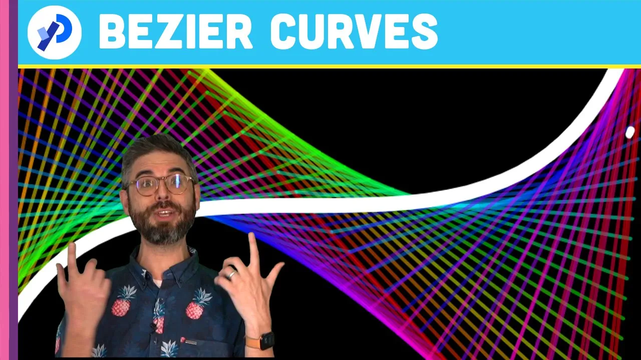
Bézier curves (Coding Challenge 163)
289K
Linear interpolation (LERP) is a fundamental mathematical operation that takes two values and returns a value somewhere between them based on a percentage (t) ranging from 0 to 1. For example, if t = 0.5, LERP returns the midpoint between the two values. The formula works by starting at the initial value and adding t times the difference between the final and initial values. In code, this is implemented as: result = start + (end - start) × t. LERP is essential for creating smooth transitions and forms the basis for constructing Bézier curves.
Click to watch →

Essential Mathematics For Aspiring Game Developers
426.9K
Linear interpolation finds intermediate values between two endpoints based on a percentage parameter t (ranging from 0 to 1). The formula is: result = start + (end - start) × t. When t=0, the result equals the start value; when t=1, it equals the end value. This works for scalars, vectors, and multi-dimensional data. In games, this enables smooth transitions between positions, colors, or any numerical values over time.
Click to watch →

Geometric Algebra - Linear and Spherical Interpolation (LERP, SLERP, NLERP)
28.8K
Linear interpolation between two vectors V_i and V_f follows the formula V_s = (1-s)V_i + sV_f, where s ranges from 0 to 1. This creates an affine combination where coefficients sum to 1, ensuring the interpolated vector lies on the line joining the vector tips. When s=0, V_s equals V_i; when s=1, V_s equals V_f. The formula can be extended beyond [0,1] to interpolate along the extended line. This method is computationally simple but produces vectors inside the unit sphere when interpolating between unit vectors.
Click to watch →
Deep Dive
Parametric equations, specifically understanding how a curve can be defined using a parameter (usually 't' ranging from 0 to 1).
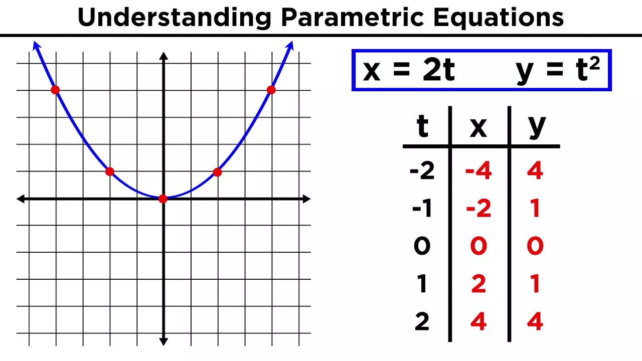
Parametric Equations
273.2K
Parametric equations define x and y coordinates as separate functions of a shared parameter (typically time), enabling independent modeling of motion components such as horizontal and vertical movement in projectile motion; these equations can be converted to rectangular form by eliminating the parameter, and vice versa, with each approach offering advantages depending on the context and graphing requirements.
Click to watch →

Parametric equations 1 | Parametric equations and polar coordinates | Precalculus | Khan Academy
950.2K
Parametric equations define x and y as separate functions of a third parameter (such as time), allowing us to describe the position of a moving object at any given moment and understand its path and direction of motion; for example, a car driving off a 50-meter cliff at 5 m/s horizontally follows the parametric equations x(t) = 5t + 10 and y(t) = 50 - 5t², which together show the car's parabolic trajectory and enable calculation of its exact position at any time.
Click to watch →

Уравнение Зоны в PUBG ☷ SHIZ
7K
A parametric curve is defined by expressing coordinates as functions of a single parameter t. For a curve, one parameter suffices because it is one-dimensional. Each value of t corresponds to a specific point on the curve.
Click to watch →
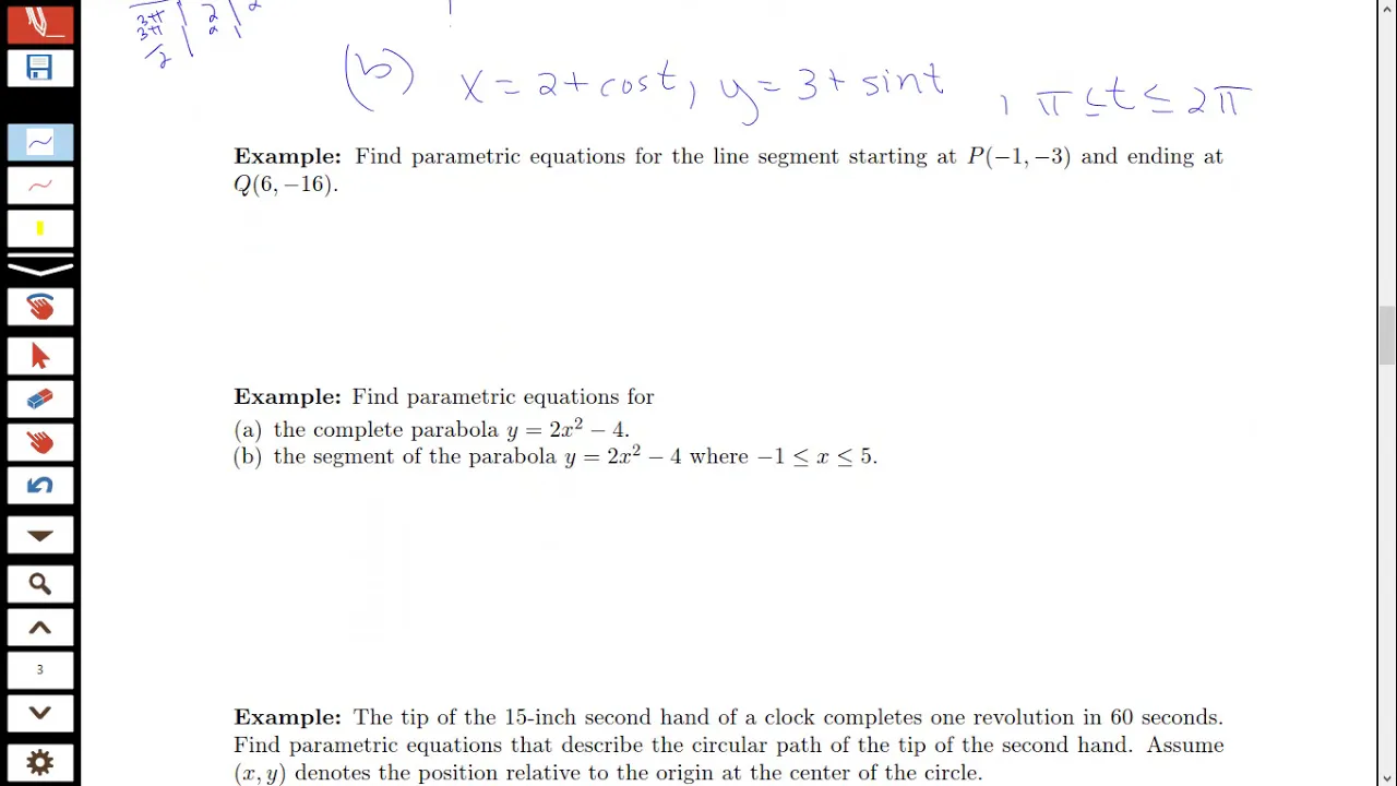
Finding parametric equations for a curve
30.3K
This video explains how to find parametric equations for curves, covering two main cases: (1) For circles, use x = x₀ + a cos(Bt) and y = y₀ + a sin(Bt) for counterclockwise tracing, or swap sine and cosine for clockwise tracing, with the interval T between 0 and 2π/|B| to trace once; (2) For lines, use x = x₀ + at and y = y₀ + bt where the slope is b/a, and adjust the T interval to trace a specific segment. Additional examples include parameterizing a parabola by letting x = t and solving for y, and modeling circular motion like a clock's second hand by determining the angular velocity coefficient B based on the desired period.
Click to watch →

Core 4 - Parametric Equations (1) - Introduction Curve sketching converting to cartesian Maths
11.4K
Parametric equations define x and y as separate functions of a third variable called a parameter (typically t or θ), unlike Cartesian equations which express y as a function of x. For example, x = 2t + 1 and y = 3t² - 4 are parametric equations where t is the parameter. These equations can model real-world situations like projectile motion (e.g., a tennis ball's trajectory: x = 15t, y = 2.5 - 15t²). Parametric curves can be graphed by creating a table of (x,y) values for different parameter values, and they can be converted to Cartesian form by eliminating the parameter using algebraic manipulation or trigonometric identities (e.g., x = 2cosθ, y = 2sinθ converts to x² + y² = 4, a circle). Differentiation and integration of parametric equations use the chain rule: dy/dx = (dy/dt)/(dx/dt), and ∫y dx = ∫y(t) × (dx/dt) dt.
Click to watch →
Deep Dive
Basic vector algebra, including vector addition, subtraction, and scalar multiplication.
Vector Algebra in 48 Minutes | Plus Two Maths Chapter 10 | Eduport Plus Two
191.7K
Vector addition combines corresponding components: a + b = (a₁+b₁)i + (a₂+b₂)j + (a₃+b₃)k. Subtraction follows the same pattern: a - b = (a₁-b₁)i + (a₂-b₂)j + (a₃-b₃)k. Scalar multiplication multiplies each component by a scalar k: k·a = (k·a₁)i + (k·a₂)j + (k·a₃)k. Two vectors are equal if all corresponding components are equal. These operations form the algebraic foundation for vector analysis and are essential for solving physics and engineering problems.
Click to watch →
![FÍSICA - Vectores Parte 01 [CICLO FREE]](https://i.ytimg.com/vi/ZO0GhczO6_U/maxresdefault.jpg)
FÍSICA - Vectores Parte 01 [CICLO FREE]
81K
Basic vector operations include addition (replacing multiple vectors with a resultant), subtraction (adding the opposite), scalar multiplication, and vector multiplication (scalar and vector products). Vector addition uses the same plus sign as real number addition. The resultant is the single vector that replaces the group.
Click to watch →
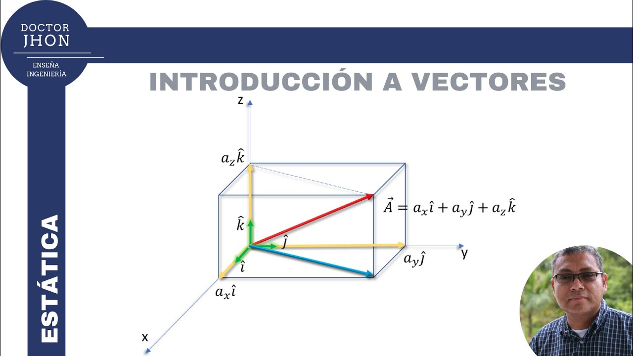
Introducción a Vectores
751
This section covers the two fundamental operations that form the basis of vector theory: vector addition and scalar multiplication. Vector addition combines two vectors to produce a resultant, with two methods: the parallelogram method (placing vectors tail-to-tail and drawing parallel lines to form a parallelogram, with the resultant as the diagonal) and the triangle method (placing vectors head-to-tail, with the resultant from the first tail to the last head). Vector addition is commutative (A + B = B + A). Scalar multiplication changes magnitude and/or sense while preserving direction: scalars >1 increase magnitude, 0<scalar<1 decrease magnitude, and negative scalars reverse sense. Vector subtraction is performed by adding the negative of the vector being subtracted: A - B = A + (-B).
Click to watch →

Unit Vector I Lecture -6 | Vector I | Class XI I Sahitya Roy (B.Tech - EE-IIT Kharagpur)
148
Vector addition involves adding corresponding components: P + Q = (P_x + Q_x)î + (P_y + Q_y)ĵ + (P_z + Q_z)k̂. Vector subtraction involves subtracting corresponding components: P - Q = (P_x - Q_x)î + (P_y - Q_y)ĵ + (P_z - Q_z)k̂. Scalar multiplication multiplies each component by the scalar: k(aî + bĵ + ck̂) = (ka)î + (kb)ĵ + (kc)k̂. For combined operations like 2a + 3b + 5c, multiply each vector by its scalar first, then add components.
Click to watch →

Vectores 1
132
Vector addition and subtraction require vectors of the same dimension, performed component-wise. Scalar multiplication by a real number t scales each component: t*(a1,a2,...,an) = (t*a1, t*a2, ..., t*an). When |t| > 1, the vector scales up; when 0 < |t| < 1, it scales down; when t = 0, the result is the zero vector; when t < 0, the direction reverses. For natural numbers, t*a equals a added to itself t times. These operations form the foundation of vector algebra.
Click to watch →
Deep Dive
Fundamental polynomial algebra, specifically expanding and manipulating quadratic and cubic equations.

10. Sınıf Matematik 2. Dönem 1. Yazılı Hazırlık Çalışması | İZLE 💯 AL! | PDF | #10sınıf
6.7K
Polynomials require non-negative integer exponents. The Remainder Theorem states that dividing P(x) by (x-a) yields remainder P(a). For quadratic equations, Vieta's formulas give sum of roots = -b/a and product = c/a. Cubic expressions expand by multiplying binomials. When two equations share a common root, express other roots and use the ratio of constant terms to find the common root.
Click to watch →

Barış Yayınları Polinom Parabol Konu Denemesi 7 (Güncel Basım)
2.8K
This comprehensive segment covers polynomial and quadratic equation fundamentals: (1) Polynomial degree operations - multiplying by x^n increases degree by n, dividing decreases by n, multiplying polynomials adds degrees, dividing subtracts degrees. (2) Polynomial construction from roots using factors (x - r_i). (3) Quadratic equation solving - discriminant Δ = b² - 4ac, roots [-b ± √Δ]/(2a), root difference √Δ/|a|. (4) Factoring method for quadratics. (5) Complex numbers - √(-k) = i√k, equate real and imaginary parts. These foundational concepts enable systematic problem-solving in algebra.
Click to watch →
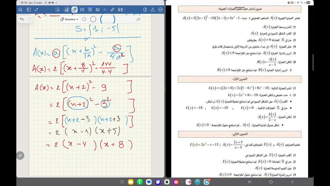
مراجعة شاملة حول العبارات الجبرية السنة الأولى ثانوي
137
A quadratic equation is written as ax² + bx + c = 0 with a ≠ 0. The discriminant (delta = b² - 4ac) determines solution nature: delta < 0 means no real solutions, delta > 0 means two distinct solutions, delta = 0 means one repeated solution. Solutions are x = (-b ± √delta)/(2a). To expand algebraic expressions: apply distributive property, combine like terms, simplify coefficients. After expansion, write in standard form (x + b/(2a))² - delta/(4a²). For 3(2x - 1)² - 10(2x - 1) + 4x² - 1, this simplifies to 16x² - 32x + 12, which becomes (x - 1)² - 16.
Click to watch →

Lecture | Algebra | Quadratic Equation | Cubic | Polynomial | JEE Main and Advanced | by Gautam Sir
147
For a cubic equation x³ + px² + qx + r = 0 with roots α, β, γ, the sum of roots (α + β + γ) equals -p, the sum of products of roots taken two at a time (αβ + βγ + γα) equals q, and the product of roots (αβγ) equals -r. For a polynomial equation of degree n with roots α₁, α₂, ..., αₙ, the sum of all roots equals -a(n-1)/aₙ, the sum of products of roots taken two at a time equals a(n-2)/aₙ, and the product of all roots equals (-1)ⁿ × a₀/aₙ. Complex roots of polynomial equations with real coefficients always occur in conjugate pairs, meaning if a + bi is a root, then a - bi must also be a root.
Click to watch →
▶️GÜVƏN BURAXILIŞ SINAQ 7 | #riyaziyyat #buraxilisimtahani #2023 #sertifikasiya #qəbulimtahanı
669
This segment covers polynomial expansion and quadratic equation concepts including perfect square trinomials (a + b)² = a² + 2ab + b², cubic expression expansion (x + 2)³ = x³ + 6x² + 12x + 8, and quadratic equation root relationships (sum of roots = -b/a, product of roots = c/a). The content demonstrates how to expand polynomial expressions, recognize perfect square trinomials, and use the relationships between coefficients and roots to solve quadratic equations without finding individual roots. These algebraic techniques are fundamental for higher-level mathematics.
Click to watch →
Prerequisite Knowledge
- Concept 01The concept of linear interpolation (LERP) and how to calculate a point between two coordinates.
- Concept 02Parametric equations, specifically understanding how a curve can be defined using a parameter (usually 't' ranging from 0 to 1).
- Concept 03Basic vector algebra, including vector addition, subtraction, and scalar multiplication.
- Concept 04Fundamental polynomial algebra, specifically expanding and manipulating quadratic and cubic equations.
Subsequent Learning
- Step 01De Casteljau's algorithm, the recursive geometric method used to evaluate and subdivide Bezier curves.
- Step 02Spline continuity conditions (C0, C1, C2 and G0, G1, G2 geometric continuity) for smoothly joining multiple Bezier curves together.
- Step 03B-Splines and Non-Uniform Rational B-Splines (NURBS), which generalize Bezier curves for advanced 3D modeling.
- Step 04Practical applications in computer graphics and design, such as vector font rendering, SVG path generation, and camera path interpolation in game engines.
Curve Basics
Cubic Curves
Curve Basics
0:00Playing Section
- 1
Explains Bezier curves using control points for smooth scalable paths.
- 2
Covers linear interpolation as the foundation for curve construction.
NURBS and B-Splines: Overcoming the Limitations of Bezier Curves
While Bezier curves are foundational in computer graphics, they possess significant mathematical limitations. Most notably, they lack 'local control'—meaning that modifying a single control point alters the entire curve, making complex designs tedious to edit. Furthermore, standard Bezier curves cannot precisely represent conic sections, such as perfect circles or ellipses, without approximation. To address these drawbacks, B-Splines and Non-Uniform Rational B-Splines (NURBS) are utilized as superior alternatives. B-Splines introduce localized control, ensuring that adjusting one control point only deforms a specific segment of the curve. NURBS expand on this by introducing mathematical weights to control points, allowing for the exact representation of both free-form geometry and standard analytical shapes like spheres and cylinders. Consequently, while Bezier curves remain popular for simple 2D vector art and fonts, NURBS have become the industry standard for computer-aided design (CAD) and high-precision 3D modeling.
Deep Dive
De Casteljau's algorithm, the recursive geometric method used to evaluate and subdivide Bezier curves.

Lecture 03 (Part 02)
240
De Casteljau's algorithm is a recursive method for generating Bezier curves. It uses notation Pᵢ⁰ for original control points. The algorithm recursively computes intermediate points: Pᵢʲ = (1-t)Pᵢ⁺ⱼ⁻¹ + tPᵢ₊₁⁺ⱼ⁻¹, where j represents the layer number. The final point P₀ⁿ is the point on the curve. This algorithm provides a geometric interpretation of curve generation.
Click to watch →

Curves
3.5K
The de Casteljau algorithm constructs a Bezier curve point for a given parameter t: (1) Compute Q₀ = (1-t)P₀ + tP₁, Q₁ = (1-t)P₁ + tP₂, Q₂ = (1-t)P₂ + tP₃. (2) Compute R₀ = (1-t)Q₀ + tQ₁, R₁ = (1-t)Q₁ + tQ₂. (3) Compute S = (1-t)R₀ + tR₁. This point S lies on the Bezier curve for parameter t. The algorithm can be extended to higher-order curves. This recursive process generates points on the curve by repeatedly interpolating between adjacent points.
Click to watch →

Computer Graphics Unit 4 One shot BCS053 | Curves and Surfaces Unit 4 Computer Graphics AKTU BCS053|
23.1K
The de Casteljau algorithm calculates points on a Bezier curve through recursive linear interpolation: Q₀ = (1-u)P₀ + uP₁, Q₁ = (1-u)P₁ + uP₂, Q₂ = (1-u)P₂ + uP₃, then C₁ = (1-u)Q₀ + uQ₁, C₂ = (1-u)Q₁ + uQ₂, and finally R = (1-u)C₁ + uC₂. To solve Bezier curve problems numerically: assume a number of steps, calculate u increment (Δu = 1/n_steps), calculate u values from 0 to 1, calculate blending function values, calculate the Bezier polynomial, and substitute control point coordinates to find x and y coordinates. A key property is that Bezier curves always pass through the first and last control points.
Click to watch →
![[Part 2/6] C# Scripting and Plugin Development for Grasshopper](https://i.ytimg.com/vi_webp/urWRRpy1fCw/maxresdefault.webp)
[Part 2/6] C# Scripting and Plugin Development for Grasshopper
31.7K
In the De Casteljau algorithm, when a curve segment is not close enough to the actual curve, it is subdivided into two halves. The subdivision is done by computing the midpoint T-value (average of start and end T-values) and recursively calling the function for the first half (start to midpoint) and the second half (midpoint to end). This process continues until all segments are within the specified tolerance. The midpoint calculation is: (startT + endT) / 2.
Click to watch →
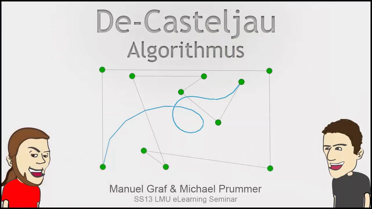
Bezier Kurven berechnen mit dem Decasteljau Algorithmus
7.5K
The de Casteljau algorithm is a recursive method for calculating points on Bezier curves by repeatedly dividing the segments between control points in a specified ratio (typically 1:1 for the midpoint), where each division creates new points that form a new control polygon, and this process continues until a single point remains on the curve; the algorithm can be implemented in Java using nested loops that calculate new points by combining adjacent points weighted by the parameter t and (1-t), with more division steps resulting in a smoother curve approximation.
Click to watch →
Deep Dive
Spline continuity conditions (C0, C1, C2 and G0, G1, G2 geometric continuity) for smoothly joining multiple Bezier curves together.
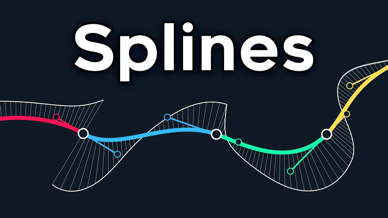
The Continuity of Splines
1.8M
Continuity measures how smoothly curves connect at joins. C⁰ continuity requires position continuity (no jumps). C¹ continuity adds velocity continuity (first derivative), requiring mirrored tangent points. C² continuity adds acceleration continuity, progressively constraining control points and reducing local control. C³ continuity is impossible for cubic Béziers without losing all control. Geometric continuity (Gⁿ) focuses on shape rather than parameterization: G¹ requires tangent direction continuity (normalizing velocity), G² requires curvature continuity (osculating circles), and G³ requires curvature rate continuity. Regular curves (non-zero velocity) satisfy Cⁿ → Gⁿ, but cusps violate this. Reflection seams in industrial design require G² continuity.
Click to watch →
Parametric & Geometric Continuity Condition:Zero order, First order & Second order!
26K
When joining two parametric curve pieces, parametric continuity (C0, C1, C2) requires matching parameter values, first derivatives, and second derivatives respectively at the joining point, while geometric continuity (G0, G1, G2) requires matching endpoints, proportional tangent vectors, and proportional curvature vectors respectively, with geometric continuity being a visual requirement that does not necessarily imply parametric continuity.
Click to watch →

Lecture 34 - Computer Graphics - Cubic Spline Curve - Deepali Jaadhav
800
Geometric continuity conditions deal with the shape of the curve rather than the parametric representation. Zero order geometric continuity (G⁰) is the same as zero order parametric continuity - the curves must have the same coordinate position at the boundary point. First order geometric continuity (G¹) means the first parametric derivatives are proportional to each other at the intersection point, not necessarily equal. The tangent vector direction must be the same, but the magnitude may differ based on a constant k. Second order geometric continuity (G²) means both first and second order parametric derivatives are proportional at the boundary point.
Click to watch →

Introduction to Computer Graphics, Lecture 3: Curves and surfaces
3.8K
This section presents the formal conditions for joining cubic Bézier curves with different levels of smoothness. It distinguishes between C-continuity (parametric smoothness requiring continuous derivatives as functions of parameter t) and G-continuity (geometric smoothness requiring matching geometric properties regardless of parameterization). For C0 continuity, curves share one control point. For G1 continuity, edge vectors must be parallel. For C1 continuity, edge vectors must be identical. For G2 continuity, non-linear conditions on the first three control points apply. The section emphasizes that C1 implies G1 for regular curves, but G1 does not imply C1, highlighting the importance of understanding both perspectives in geometric modeling.
Click to watch →
![[CPE630] CAGD - Introduction to Computer Aided Geometric Design EP.1](https://i.ytimg.com/vi/DOotnTN0dR0/sddefault.jpg)
[CPE630] CAGD - Introduction to Computer Aided Geometric Design EP.1
1.2K
This section presents the mathematical criteria for joining curves smoothly. C₀ continuity requires matching endpoints (Q₁(1)=Q₂(0)), ensuring curves meet at a common location. C₁ continuity adds matching tangent vectors (Q₁'(1)=Q₂'(0)), producing visually smooth transitions. G₁ continuity relaxes this to require only matching tangent directions (Q₁'(1)=k×Q₂'(0)), allowing different magnitudes. These continuity conditions form the basis for constructing complex curves from simpler segments while maintaining desired smoothness properties.
Click to watch →
Deep Dive
B-Splines and Non-Uniform Rational B-Splines (NURBS), which generalize Bezier curves for advanced 3D modeling.

Curves and Surfaces
15.4K
NURBS (Non-Uniform Rational B-Splines) generalize Bezier curves by automatically handling piecewise construction and providing smooth connections between segments. They require specifying order (degree+1), degree, and knot sequences. Uniform knots produce evenly spaced parameters, while non-uniform sequences enable custom spacing. Repeating knots forces curves through specific points. NURBS combine the mathematical rigor needed for industrial applications with the flexibility of arbitrary control point arrangements, forming the backbone of professional CAD and animation software.
Click to watch →

Lec-47 B-Spline Curve
127.1K
B-spline curves offer significant advantages over Bezier curves by allowing independent specification of curve order (k) from the number of control points, enabling local propagation where changing a control point affects only nearby segments rather than the entire curve. The curve is composed of n-k+2 segments with C^(k-2) continuity, where k=3 provides slope continuity and k=4 provides curvature continuity. NURBS (Non-Uniform Rational B-splines) extend B-splines by introducing weights to control points, enabling exact representation of conic sections like circles, ellipses, parabolas, and hyperbolas, which cannot be achieved with standard B-splines or Bezier curves. This mathematical flexibility makes NURBS the industry standard for representing curves and surfaces in computer-aided design.
Click to watch →

B Spline Curve - Techniques For Geometric Modeling - CAD/CAM/CAE
5.1K
B-splines of order k are piecewise polynomials of degree k-1 with C^(k-2) continuity. Knot vectors define the intervals where basis functions are non-zero, with uniform versions having equally spaced knots. NURBS extend B-splines by introducing non-uniform knot vectors and rational weights w_i, providing additional design freedom. These weights enable exact representation of conic sections and combine the strengths of B-splines and Bezier curves. NURBS have become the industry standard for CAD data exchange due to their versatility in representing complex shapes with precise mathematical control.
Click to watch →
![ĐỒ HỌA MÁY TÍNH [BUỔI 3]](https://i.ytimg.com/vi/u0wgtv4C3OE/maxresdefault.jpg)
ĐỒ HỌA MÁY TÍNH [BUỔI 3]
1.2K
B-Splines improve upon Bezier curves by providing local control, where each control point affects only a portion of the curve. NURBS (Non-Uniform Rational B-Splines) extend B-Splines by incorporating rational weights, enabling exact representation of conic sections. These techniques are essential for CAD applications and high-quality 3D modeling, providing flexibility in representing complex shapes while maintaining computational efficiency.
Click to watch →
The Continuity of Splines
1.8M
Non-Uniform Rational B-Splines (NURBS) extend B-splines by allowing control of the priority or weight of each control point, making curves gravitate toward or away from specific points. They also support non-uniform knot intervals. NURBS are particularly powerful because they can represent conic sections exactly, including perfect circles, which is crucial for precise geometric modeling.
Click to watch →
Deep Dive
Practical applications in computer graphics and design, such as vector font rendering, SVG path generation, and camera path interpolation in game engines.
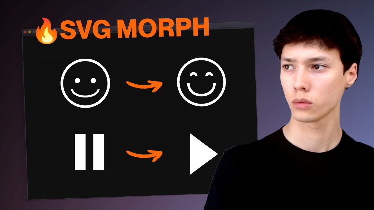
How to Morph an SVG using Framer Motion, Flubber.js and Nextjs
19.5K
The flubber.js library provides an interpolate function that calculates intermediate paths between two SVG paths. The interpolator takes two path 'd' attributes as input and returns a new path at any given progress value between 0 and 1. A progress value of 0 returns the original path, 1 returns the target path, and values in between produce intermediate shapes. This allows developers to morph between any two SVG shapes by calculating the mathematical approximation of their transformation.
Click to watch →
Автоматический дизайн · Доклад, 2021
5.5K
SVG (Scalable Vector Graphics) is an XML-based format ideal for automated design generation. Unlike PDF with its complex internal structures, SVG uses text-based tags describing shapes and paths. To use fonts, you must convert font glyphs to SVG path data using specialized libraries. This allows programmatic generation of vector graphics with any font, enabling automated design production.
Click to watch →

Fourier Analysis For The Rest Of Us
47.6K
This section covers the practical aspects of extracting mathematical equations from vector graphics. Vector graphics store drawing instructions rather than pixel data, enabling lossless scaling unlike raster formats. SVG files contain path data as strings of letters followed by coordinates: 'M' moves to a point, 'Q' draws quadratic Bézier curves, and 'L' draws lines. Each new instruction implicitly starts at the previous endpoint, creating compact but cryptic representations requiring parsing. Quadratic Bézier curves are defined by three points (initial, control, final) with parametric equation B(t) = (1-t)²P₀ + 2(1-t)tP₁ + t²P₂. Programming implementation involves importing raw SVG text, parsing instructions, explicitly recording starting points, translating coordinates to center shapes, inverting y-axis, and pairing x/y coordinates for proper data structure organization.
Click to watch →

NV_path_rendering Introduction (Part 1)
3K
NV_path_rendering is an OpenGL extension that implements GPU-accelerated path rendering using a stenciled in-cover (STC) approach, where paths are first stenciled into the stencil buffer and then covered with conservative geometry, enabling efficient rendering of resolution-independent 2D vector graphics with support for all major path rendering standards including dashing, join styles, text, and font rendering, while allowing integration with traditional 3D rendering pipelines.
Click to watch →

Mod Deep Dives - CMDCam
14K
CMDCam is a Minecraft mod that enables precise camera control for video production by allowing users to define paths that the camera follows, with different interpolation methods (linear, hermite, cubic, cosine) determining how smoothly the camera moves between points, and target settings (direct or indirect) controlling what the camera focuses on during the animation.
Click to watch →
Curve Basics
Cubic Curves
Curve Basics
0:00- 1
Explains Bezier curves using control points for smooth scalable paths.
- 2
Covers linear interpolation as the foundation for curve construction.
NURBS and B-Splines: Overcoming the Limitations of Bezier Curves
While Bezier curves are foundational in computer graphics, they possess significant mathematical limitations. Most notably, they lack 'local control'—meaning that modifying a single control point alters the entire curve, making complex designs tedious to edit. Furthermore, standard Bezier curves cannot precisely represent conic sections, such as perfect circles or ellipses, without approximation. To address these drawbacks, B-Splines and Non-Uniform Rational B-Splines (NURBS) are utilized as superior alternatives. B-Splines introduce localized control, ensuring that adjusting one control point only deforms a specific segment of the curve. NURBS expand on this by introducing mathematical weights to control points, allowing for the exact representation of both free-form geometry and standard analytical shapes like spheres and cylinders. Consequently, while Bezier curves remain popular for simple 2D vector art and fonts, NURBS have become the industry standard for computer-aided design (CAD) and high-precision 3D modeling.
The concept of linear interpolation (LERP) and how to calculate a point between two coordinates.
Parametric equations, specifically understanding how a curve can be defined using a parameter (usually 't' ranging from 0 to 1).
Basic vector algebra, including vector addition, subtraction, and scalar multiplication.
Fundamental polynomial algebra, specifically expanding and manipulating quadratic and cubic equations.
De Casteljau's algorithm, the recursive geometric method used to evaluate and subdivide Bezier curves.
Spline continuity conditions (C0, C1, C2 and G0, G1, G2 geometric continuity) for smoothly joining multiple Bezier curves together.
B-Splines and Non-Uniform Rational B-Splines (NURBS), which generalize Bezier curves for advanced 3D modeling.
Practical applications in computer graphics and design, such as vector font rendering, SVG path generation, and camera path interpolation in game engines.
247K views7.8Klikes3:04@GuidevOriginal Release: 2018-03-22
hello everyone busy curves are used to draw smooth curves that can be scaled indefinitely I will be doing a lot of tutorials where I will be using them so I thought maybe I should make a video explaining them so you can have an idea of what it is all about that busy acres is defined by a set of control points for example to draw a line segment we need two points in this case p0 and p1 to get any point in these segments we use a linear physical function which is equivalent to a linear interpolation with t varies from 0 to 1 this function simply means that the influence of each point depends on T for T equal to 0 we will get p 0 for t equal to 1 we will get P 1 and for each value between 0 & 1 we will get a point along the line segment linking p 0 and P 1 here is a visualization of how it works great that was pretty simple now what about drawing a curve in this case we need three points and use a quadratic PC curve first we need to do another linear interpolation between p1 and p2 and then interpolate between L 0 and L 1 this will give us Q 0 if we trace the path of Q 0 it will show a curve going from the first points to the last point the first and the last control points are always the end points of the curve this function can also be rewritten into this form this is what is known as a quadratic Bezier curve for a cubic Bezier curve we need to add another control points P 3 we do a linear interpolation between P 2 and P 3 we call it L 2 we do another interpolation between l1 and l2 and finally we interpolate between q0 and q1 if we tracy zeros but it will look like this we can rewrite the function into this form and this is what is known as a cubic busy curve so after all quadratic Bezier curve is just an interpolation between two linear interpolations and the cubic busy curve is an interpolation between two quadratic curves I hope this video helped you understand the basics of busy curves thanks for watching and don't forget to leave your feedback and subscribe see you next time
Up Next

77:03
Python Programming Basics for Beginners | Crash Course Tutorial
@MatthewMYoung
1K views•2021-06-08
87:26
Introduction to Secure Multiparty Computation with Yehuda Lindell
@fhe_org
7.7K views•2021-02-04

4:55
HTTP Requests Explained: GET, POST, PUT, DELETE
@codecademy
103.1K views•2021-10-07

19:25
Enigma Machine Mechanics: WWII Encryption Explained
@JaredOwen
13.2M views•2021-12-11
Related Study Plans & Knowledge Roadmaps
Structured learning paths in Computer Science
computer-science
Container Runtimes: Namespaces, Cgroups & Go
01Linux Systems & Go Programming Foundations
02The Core of Isolation: Chroot and Filesystems
03Linux Namespaces: Process Isolation
+ 3 more learning modules
32h6 modules
Explore Roadmap
computer-science
Building a CHIP-8 Emulator: Rust & CPU Basics
01Computer Architecture Foundations (Bits & Bytes)
02Rust Programming for Systems Development
03CHIP-8 Virtual Hardware Specifications
+ 2 more learning modules
32h5 modules
Explore Roadmap
computer-science
Building BitTorrent: Go, P2P & Concurrency
01Go Fundamentals & Concurrency
02Networking Foundations & P2P Architecture
03Bencode Parsing & Torrent Metadata
+ 3 more learning modules
26h6 modules
Explore Roadmap
computer-science
Actor Models (C++ Concurrency & Lock-Free)
01C++ Multi-Threading Foundations
02Thread Pools and Task Scheduling
03Atomics and Lock-Free Queue Design
+ 3 more learning modules
45h6 modules
Explore Roadmap