Graph Representation in Python: Tuples, Adjacency Lists & Matrices (Tutorial)

[00:00:00]hey there and welcome to part two of graph theory with python my name is david amos in this video i'm going to show you how to represent graph data structures using the python programming language if you haven't already seen my video on the origins of graph theory i'll put a link to it right up here before i show you how to represent a graph data structure in python i need to talk a little bit about the precise definition of a graph in mathematics a graph which we'll denote with a capital letter g is a pair of two sets v and e the set v is called the vertex set and the set e is called the edge set now if you don't know what a set is you can think of it as a collection of distinct objects although you'll see in a little bit that we're going to use this a little bit loosely we can actually in some cases have multiple objects in a set if you're interested i have a video on some of the weird things that can happen when you aren't careful about how you define a set i'll put a link on the screen and also down in the description for our purposes though we're just going to think of the sets of v and e as collections of objects now the vertices of a graph can be any object we want they could be people in a social network they could be items manufactured by a company they could be mathematical objects like functions or they could be python objects like integers or strings in the vast majority of examples we'll look at we're going to take our vertices from the natural numbers including zero so for example we could have a graph with a vertex set containing the numbers 0 1 2 and 3. the edge set of a graph is a collection of pairs of vertices for example we could have an edge set with the pairs 0 1 0 2 1 3 and 2 3.

[00:01:56]now from a mathematical standpoint this is all a graph is a vertex set and an edge set that's not very intuitive though and we often represent graphs graphically using dots for the vertices and lines connecting the dots to represent edges let's draw the graph represented by our vertex set v in edge set e that we have here we have four vertices and i'll go ahead and label them 0 1 2 and 3. we also have four edges we have the edge 0 1 which i can draw by connecting vertex 0 to vertex 1. we have the edge 0 2 which i can draw by connecting the vertex 0 to the vertex 2 the edge 1 3 which is this edge and the edge 2 3 which is this edge here it's important to remember that the way that a graph is drawn doesn't influence the nature of the graph itself what i mean by that is i could draw the graph this way i could label this vertex 0 this vertex 1 this vertex 2 and this vertex 3.

[00:02:57]now when i draw my four edges there's the edge 0 1 the edge 0 2 the edge 1 3 and the edge 2 3. i've drawn this graph in such a way that the lines do not cross here in the center like they did in the first drawing but it is still the same graph i could even get a little crazier if i wanted to for example i could draw the four vertices in a straight line here's 0 1 2 3 and draw my edges like this here's 0 1 here's 0 2 here's 1 3 here's 2 3.

[00:03:30]this is another way to represent the same graph graphically there are some other things that can happen in graphs such as two vertices having multiple edges between them and one vertex having an edge connected to itself let me show you what i mean here's a graph representing the seven bridges of konigsberg from the first video in the series let's label the vertices a b c and d the vertices a and b have two edges between them the same for a and c a graph with this property is called a multi-graph let's write out the vertex set v in edge set e for the konigsberg graph v is the set of the four vertices a b c and d our edge set e has seven edges which if you saw the first video in the series you'll recognize as the seven bridges from the city of konigsberg they are a b which can be this edge here a second edge between a and b which is this edge two edges between a and c which gets us these two edges here an edge between b and d an edge between a and d and an edge between c and d this is where we're abusing the notion of a set a little bit we have two copies of the edge a and b and two copies of the edge ac now in a real set we couldn't have multiple copies of the same object a set like this is usually called a multi-set in some cases a graph can have an edge between a vertex and itself we call these edges loops and here's an example of one on this graph let's write out the vertex and edge sets for this graph our vertex set v again has four elements zero one two and three and our edge set has six elements we have the edge zero zero representing the loop the edge zero one the edge zero three the edge one three the edge one two and the edge two three now mathematicians study graphs for lots of reasons they're incredibly useful as models for relationships between objects a great example that most people are familiar with is a social network such as facebook or linkedin in facebook for example the vertices are the people who are members of facebook edges represent the friendship relation between facebook friends now that you've seen how we represent a graph mathematically let's take a look at how we can represent this in python first i want to mention a little bit about the version of python that i'm going to be using and that you should use to follow along successfully i'm using python 3.9.1 most everything that we'll be doing in this video series can be done using python 3.6 or greater in a couple of rare instances it'll be helpful to have python 3.8 or better if you need a resource for getting the latest version of python installed on your system i highly recommend real python's python installation guide i'll drop a link to that in the video description i'm also using microsoft's visual studio code editor this is my preferred editor but by no means you have to use it in order to follow along use the editor you love the most now remember that mathematically a graph is a pair containing a vertex set and an edge set the notation that mathematicians use to represent this pair looks a lot like a common python data structure the tuple we could use a tuple to represent a graph but we're going to take it one step further and use something called the named tuple from the collections module let me go ahead and import that now name tuples are great for creating blueprints that you can use to instantiate new objects they work a lot like a tuple except that they allow you to give names to the tuple's components once you've created a name tuple you can use it to create new instances of objects much the same way you would using a user-defined class to create our graph type we start by assigning a named tuple to the named graph with a capital g the first thing we have to pass to namedtuple is a string containing the name of the type which for us is just graph with a capital g the next thing you have to pass to name tuple is a string or an iterable containing the field names now i prefer to use an iterable like a list with strings containing the field names these will be the names of the components of the tuple for graphs that would be vertices and edges mathematicians commonly refer to vertices in graphs however computer scientists often prefer the name nodes they're really the same thing nodes is a little bit shorter and easier to write so i'm going to use that instead of vertices in our graph type now that we've created the graph name tuple we can use it to start instantiating graph objects let's create one representing the konigsberg graph that we saw earlier i'll put that picture side by side with my editor window so we can refer to it while we're instantiating the graph the konigsberg graph has four vertices a b c and d we'll use python strings to represent each node in a list to represent our collection of nodes we'll assign the list to a variable name called nodes there are seven edges in the konigsberg graph we'll use a tuple to represent each edge and store them in a list assigned to a variable called edges there are two edges between the nodes a and b this edge and this one there are also two edges between the nodes a and c this edge and this one we have one edge between the nodes a and d this edge here one edge between the nodes b and d this edge here and one edge between the nodes c and d this edge here to create a graph object representing the konigsberg graph we'll pass our nodes list and our edges list to the graph name tuple we created earlier let's call it capital g now we've created a graph data type based exactly on the mathematical definition of a graph that's great but it's not going to be the best way to represent a graph for certain kinds of problems for example if you saw my first video in the graph theory with python series we talked about how euler solved the problem of whether or not there exists a continuous walk through the city of konigsberg that uses each bridge exactly once now euler proved that this was impossible but if we tried to construct such a walk using this graph data type we've defined we'd have to do a lot of looping over the edges list this is terribly inefficient so while this data type is convenient for entering information about a graph it's not the best representation for actually doing something with a graph there are two other kinds of representations commonly used in graph algorithms the adjacency list and the adjacency matrix let's take a look at what each of those are the first representation we'll look at is called the adjacency list you can think of an adjacency list as a list of lists each list in this list of lists represents a single node in the graph and the list corresponding to each node lists all of the nodes that are adjacent to that node by adjacent we mean connected to that node by an edge so for example in the konigsberg graph node a is adjacent to node b two times because there are two edges connecting a to b so we'll list it in the adjacency list twice a is also adjacent to c twice because there are two edges connecting a to c it's also adjacent to node d node b is adjacent to a twice because there are two edges connecting a and b and it's also adjacent to node d node c is adjacent to a twice and also adjacent to node d finally node d is adjacent to node a node b and node c one thing you can notice about the adjacency list right off the bat is that it doesn't require as many characters to write out as the standard mathematical representation of a graph that's because we list the node at the beginning and then each node that it's connected to in its adjacency list without having to repeat that node multiple times for each edge also notice that how i've written this is by putting each of the four nodes followed by a colon and then a list containing each of the other nodes in the graph that they're adjacent to it kind of looks like a python dictionary and that's not by accident if we add some curly braces and some square brackets around each list you get a good idea of how we can represent this using python let's get back to our editor and write a function that takes a graph instantiated using the graph name tuple we defined earlier and returns an adjacency list as a python dictionary we're going to write a function that returns the adjacency list representation of a graph but the word list means something in python and it's not the same thing as an adjacency list as you've seen we can use a dictionary to represent the adjacency list so we're going to call our function adjacency dict this function will take one parameter a graph now all python functions should have a doc string so i'm going to go ahead and write one now the first thing we'll do is create a dictionary that we'll use to hold the adjacency list representation i'm going to call that dictionary adj for adjacency the keys of this dictionary are the nodes of the graph and the values are lists of adjacent nodes let's create this using a dictionary comprehension each key will be a node and we'll start each value as an empty list we need to do this for each node in the graphs node list next we're going to loop over all of the edges in the graph let's take the two nodes in each edge and assign them to variables called node 1 and node 2. since there's an edge between node 1 and node 2 node 2 is adjacent to node 1 which means we need to append node 2 to node 1's adjacency list on the other hand node one is adjacent to node two so we also need to append node one to node two's adjacency list when this for loop completes we'll have a dictionary with one key for each node in the graph and a list containing all the nodes adjacent to each node that's exactly the adjacency list representation so we can go ahead and return this dictionary let's run our code and see what we get as the adjacency dict for the conicsberg graph we defined earlier my code is stored in a file called graph.py i'm going to run this with the i flag or interactive flag that's going to execute all of the code in dot py and then drop me into a python shell where i can interact with everything that's been executed now we created a graph called g representing the konigsberg graph let's take a look at that it has four nodes a b c and d and the seven edges from the konigsberg graph let's pass that to the adjacency dict function the dictionary returned by adjacency dict has four nodes a b c and d and lists containing all of the adjacent nodes if you compare it to the adjacency list we wrote when i told you what an adjacency list is you'll see they're the same a is adjacent to b twice to c twice and also to node d b is adjacent to a twice and also adjacent to node d c is adjacent to a twice and also node d and d is adjacent to nodes a b and c our adjacency dick function is working beautifully there's something important we need to talk about though using a dictionary to represent the adjacency list representation has an important consequence for nodes in our graph nodes are used as dictionary keys and in order to be a dictionary key nodes have to be of a hashable type one of the prerequisites for being hashable is immutability so for example things like strings or integers even tuples are fine but lists dictionaries and most user-defined classes are mutable and therefore not hashable so they can't be nodes in our graphs in practice this might be a pretty severe limitation but for our purposes we're just trying to learn some graph theory we're going to use integers and strings for nodes in all of our graphs which means we won't run into any problems when calling our adjacency dict function the adjacency matrix represents a graph as a matrix or a two-dimensional array each row and column of the matrix corresponds to a node in the graph we write a matrix as an array of numbers enclosed in two square brackets the matrix has one row for each node in the graph and one column for each node in the graph at the intersection of a row and a column for example the row corresponding to b and the column corresponding to a we record the number of edges between those two nodes since there are two edges connecting a and b in the graph we'll write down the number 2.

[00:17:35]let's fill out the first row of the konigsberg graphs adjacency matrix there are no edges connecting a to itself so we'll put a 0 at the intersection of the first row in the first column there are two edges connecting a to b so we'll put a 2 at the intersection of the first row in the second column there's also two edges connecting a and c so we'll put a 2 at the intersection of the first row in the third column finally there's one edge connecting a to d so we'll put a 1 in the last column of the first row as an exercise you might want to pause the video and see if you can fill out the rest of the adjacency matrix on your own then unpause the video and check your work got it let's see how you did let's finish filling out the second row there aren't any edges connecting b to itself so we put a zero in the second row and second column there are no edges connecting b to c so we put a zero in the second row and third column there is an edge connecting b to d so we put a one in the last column of the second row the third row corresponds to node c there are two edges connecting c to a so we'll put a 2 in the first column there are no edges connecting c to b so we'll put a 0 in the second column there aren't any edges connecting c to itself so we'll put a 0 in the third column and there's one edge connecting c to d so we'll put a 1 in the last column there's one edge between d and each of the vertices a b and c so we'll put ones in the first three columns and since d isn't connected to itself we'll put a 0 in the last column now that we know how to construct the adjacency matrix let's head back to our editor and see if we can write a function that returns the adjacency matrix for a given graph i'm going to write a function that returns the adjacency matrix for a graph let's call that function adjacency matrix the function will have one parameter a graph and i'll go ahead and give it a doc string we'll use a python list to represent the adjacency matrix and i'll assign it to a variable called adj since the adjacency matrix is a two-dimensional array each element of this list will be another list representing each row in the adjacency matrix and we need one for each node in the graph it's going to be really useful to initialize each entry in the matrix with a zero let's go ahead and do that by using a nested list comprehension now that our adjacency matrix is initialized with zeros let's loop over each edge of the graph and add values as necessary the first thing we'll do is extract the two nodes in the edge and assign them to variables called node one and node two in order to record this edge in the adjacency matrix we need to add 1 to the 0 in the row corresponding to node 1 and the column corresponding to node 2.

[00:20:28]but there might be a problem if the nodes are integers ranging from 0 up to 1 less than the number of nodes then we'll be fine they correspond to the indices in the adj list of lists however if the nodes are strings or integers that aren't in the right range then we're going to have a problem now we could use the python list index method to get the index of node 1 and node 2 in the graphs node list but for really big graphs that's going to be pretty inefficient instead we're just going to assume that the nodes are defined as integers in the range 0 up to 1 less than the number of nodes let's document that in our docs string with that assumption taken care of we can go ahead and start filling out values in the adjacency matrix since node 2 is adjacent to node 1 we need to add a 1 to the 0 in the row corresponding to node 1 and the column corresponding to node 2.

[00:21:26]and since node 1 is adjacent to node 2 we also need to add a 1 to the 0 in the row corresponding to node 2 and the column corresponding to node 1.

[00:21:37]when this for loop completes we'll have a 2 dimensional array with 0's in each position where the row node and column node aren't connected by an edge and the number of edges in each position where the row node and column node are connected by one or more edges that's exactly the adjacency matrix so we can go ahead and return adj let's go ahead and run the code and see how it works i'll use interactive mode again to execute the code in the graph.py file to drop into an interactive shell so i can play around with the adjacency matrix function let's use the konigsberg graph again so we can check whether or not the adjacency matrix function is working as we expect we do have a problem though the way we defined the conicsberg graph before was using strings as nodes with the letters a b c and d we need to relabel the graph with integers 0 1 2 and 3. let me put that side by side with my editor window so we can use it as a reference while we're building the graph let's replace a with 0 b with 1 c with 2 and d with 3. now we can recreate the graph g so that it uses the integer nodes instead of the string nodes first we'll assign to a variable called nodes the range containing the values 0 1 2 and 3.

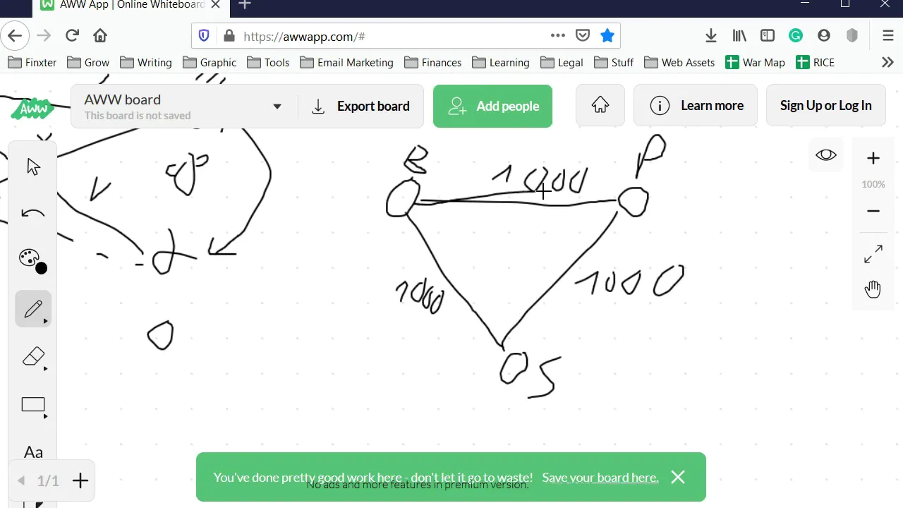
[00:22:57]next we'll assign a list to a variable called edges containing a tuple for each edge in the graph there are two edges between 0 and 1 2 edges between 0 and 2 one edge between 0 and 3 an edge between 1 and 3 and an edge between 2 and 3. now we can create a new graph using the nodes and edges lists now let's pass g to the adjacency matrix function and see what we get let's compare that to the adjacency matrix we wrote by hand and see how we did excellent the adjacency matrix function is working beautifully at this point we have three ways to represent a graph in python as a named tuple as an adjacency list or as an adjacency matrix but we've been making an assumption about the kinds of graphs we're using and it has to do with relationships remember graphs model relationships between objects we previously talked about the example of a social network like facebook on facebook the nodes are facebook accounts and an edge exists between nodes if those two accounts are friends with each other if i'm your friend on facebook you're also my friend it's a two-way relationship but that's not always the case consider a social network like instagram where accounts follow other accounts if i follow an account on instagram it doesn't necessarily mean that account follows me back the follow relationship has a direction we can separate graphs into two broad categories undirected graphs which are the kinds of graphs we've looked at so far or directed graphs which represent directed relationships the definition for a directed graph is basically the same as the definition for an undirected graph the difference is an edge in a directed graph indicates a relationship from the node at the start of the edge to the node at the end of the edge but not the other way around and when we draw directed graphs they look pretty much the same as undirected graphs the difference is we put an arrow on the edge to indicate the direction of the relationship let's take a look at how the adjacency list and the adjacency matrix differ for directed versus undirected graphs in this picture i've drawn two graphs on three vertices with the same edges on the left hand side is a directed version of the graph and on the right hand side an undirected version let's write out the adjacency list representation of the graph on the right the first thing we have to do is label our nodes we'll label them 0 1 and 2. node 0 is adjacent to node 1 and node 2 node 1 is adjacent to nodes 0 and 2 and node 2 is adjacent to nodes 0 and 1. now let's do the same thing for the directed graph on the left we'll use the same node labels 0 1 and 2 and let's write out the adjacency list representation in the directed graph node 0 is adjacent to node 2 because there is an edge with an arrow pointing towards node 2 starting from node 0.

[00:26:14]however it is not adjacent to node 1 because the edge starting at node 1 has an arrow pointing towards 0 not starting from 0 and pointing towards 1.

[00:26:25]so the adjacency list for node 0 contains a single node node 2. node 1 is adjacent to node 0 because there's an edge with an arrow starting at node 1 and ending at node 0 and adjacent to node 2 because there's an edge starting from node 1 and pointing towards node 2.

[00:26:46]node 2 isn't adjacent to anything because there are no edges coming into node 2 with arrows pointing towards it so that's a pretty big difference between the adjacency list representation of the directed and undirected graph now let's take a look at the adjacency matrix the first row of the adjacency matrix represents node 0 and so does the first column since there's no loop joining 0 to itself we put a 0 in that position the second column represents node 1.

[00:27:19]there is an edge between node zero and node one so we put a one the third column represents node two and since there's an edge between node zero and node two we put a one the second row of the matrix represents node one there is an edge between node one and node zero so we put a one in the first column there's no loop joining one to itself so we put a zero in the second column there is an edge between node one and node two so we put a 1 in the third column the final row represents node 2.

[00:27:50]there is an edge between node 2 and node 0 so we put a 1 in the first column there's an edge between node 2 and node 1 so we put a 1 in the second column but there's no loop connecting 2 to itself so we put a 0 in the third column now let's write the adjacency matrix for the directed version the first row represents node 0 and so does the first column there's no loop joining 0 to itself so we put a 0 in that position the second column represents node 1.

[00:28:23]there is no edge between node 0 and node 1 that starts at node 0 with an arrow pointing towards node 1.

[00:28:30]so we put a 0 in that position the third column represents node 2 and there is an edge between node 0 and node 2. so we put a 1 in that position the second row represents node 1. there is an edge connecting node 1 to node 0 so we put a 1 in the first position there's no edge or no loop connecting one to itself so we put a 0 in that position and there is an edge connecting one to node two so we put a one in the last position the third row represents node two there's no edge between node two and no zero so we put a zero on that position in fact there's no edges between two and any other node in the graph so we put a zero in every position in that row just like the adjacency list representation the adjacency matrix representation is pretty different let's get back to our code editor and see how we can modify our adjacency dict and adjacency matrix functions to account for directed graphs the first thing i'll do is remove the graph representation of the konigsberg graph that we created earlier just to clean things up next we need to add a field to our graph named tuple that we can use to indicate whether or not a graph is directed we'll add that to our fields list and we'll call it is directed now let's take a look at the adjacency dict function and see what we can do to modify it to account for directed or undirected graphs we don't need to change anything about the first line of the function we're still creating a dictionary whose keys are nodes and whose values are lists the change needs to happen inside of the for loop let's look at the first line we take the first component of an edge and assign it to node one and the second component of an edge and assign it to node two for a directed graph the edge starts from the first component and ends at the second component if that's the case then we still have to append node two to the adjacency list for node one so nothing needs to change on this line however this is where the problem starts if the graph is directed node 1 is adjacent to node 2 but node 2 is not adjacent to node 1 so we don't need to append node 1 to node 2's adjacency list we can skip over this line of code by adding an if statement that checks the value of is directed and executes this line of code only if is directed is set to false and that'll do it for us now let's take a look at the adjacency matrix function it's almost exactly the same we still need to initialize each entry in the adjacency matrix with zero loop over all of the edges and extract the nodes in the edges to two variables called node one and node two since this edge starts at node one and ends at node two node one is adjacent to node two so we need to keep this line however this edge does not imply that node 2 is adjacent to node 1 which means we need to put this line behind an if statement and there we go we've modified the adjacency matrix function to work with directed graphs just like before i'll run the code in interactive mode let's create a graph with three vertices for the edges let's add an edge between 1 and 0.

[00:32:00]between 1 and 2 and between 0 and 2.

[00:32:08]this is the same as the triangular looking graphs that we saw when we were comparing directed and undirected graphs let's put those on the screen so we can compare the output with what we wrote manually here's the undirected graph in order to check our functions against our previous work we need to set the is directed field to false now let's pass g to the adjacency dict function hey it worked just like it should node 0 is adjacent to nodes 1 and 2.

[00:32:43]just like we came up with earlier node 1 is adjacent to node 0 and 2 just like it should be and node 2 is adjacent to nodes 1 and 0 just like it is here let's see what happens when we pass g to the adjacency matrix function look at that it matches what we had earlier now let's set is directed to true when we try to do that we get an attribute error that says we can't set an attribute this is an important property of name tuples that i didn't mention earlier just like standard python tuples named tuples are immutable now you might be wondering wait a second but we were able to append an edge to a graph created from this named tuple what's that all about well that's because edges is a reference to a list which is a mutable object in python so even though g is an immutable object the objects in g are mutable and can be changed if that makes your head spin there's an awesome talk i got to see al swigert give at the pie cascades conference a couple years ago i'll post a link to it down in the description so since we can't change the value of is directed we'll have to create a whole new graph let's move this over so we can see the directed version of the graph and see what happens when we pass g to the adjacency dict function hey look at that it worked 0 is adjacent to node 2 just like we got earlier 1 is adjacent to nodes 0 and 2 just like it should be and 2 is adjacent to nothing its value is an empty list let's take a look at the adjacency matrix would you look at that it's exactly what it should be i love it when things work out you've now seen the precise mathematical definition of both a directed and undirected graph you learned about adjacency list representation and adjacency matrix representation and we wrote functions in python to produce these representations for us now you might be wondering why are there multiple ways to represent a graph is there a reason you'd use one over the other that's a great question let's take a look at the answer we can compare the adjacency list representation and the adjacency matrix representation from different standpoints for example one of the benefits of the adjacency list representation is that it can handle arbitrary nodes so long as those nodes are of a hashable type on the other hand the adjacency matrix only works for graphs whose nodes are integers from the perspective of amount of memory used an adjacency list typically uses less memory than an adjacency matrix especially when the graph doesn't have a lot of edges on the other hand the adjacency matrix always records data for every edge in the graph this means that no matter what you're always using the maximum amount of memory required to represent the graph for graphs with a large number of edges this isn't really a problem but if the graph is sparse meaning it doesn't have very many edges the adjacency matrix may not be the greatest choice for a representation by looking at this comparison you might be inclined to say wow it looks like the adjacency list is usually the best way to represent a graph and the answer is it really depends on what problem you're trying to solve in some cases the adjacency matrix is the perfect representation the matrix data structure lends itself to certain kinds of algorithms and certain kinds of operations thank you so much for watching all the way to the end of this video if you enjoyed it do me a favor hit the like button and share it with two people you think would like it too and if you haven't already consider subscribing to my channel tap the bell icon to get notified whenever i release a new video i'm david amos and i'll see you in the next video