













This webinar demonstrates a comprehensive workflow for extracting metagenome-assembled genomes (MAGs) from microbial community sequencing data, including quality trimming of reads, taxonomic profiling using Kaiju, metagenome assembly with multiple assemblers, differential coverage binning using MaxBin 2, MetaBAT 2, and CONCOCT, consensus binning with DAS Tool, quality assessment using CheckM, and functional annotation using GTDBtk, Species Tree, and HMMER profiling to understand organism roles in ecosystems.
Metagenome-Assembled Genome Extraction: Workflow Tutorial
Added:Fundamental concepts of metagenomics, including the differences between single-isolate sequencing and environmental shotgun sequencing.
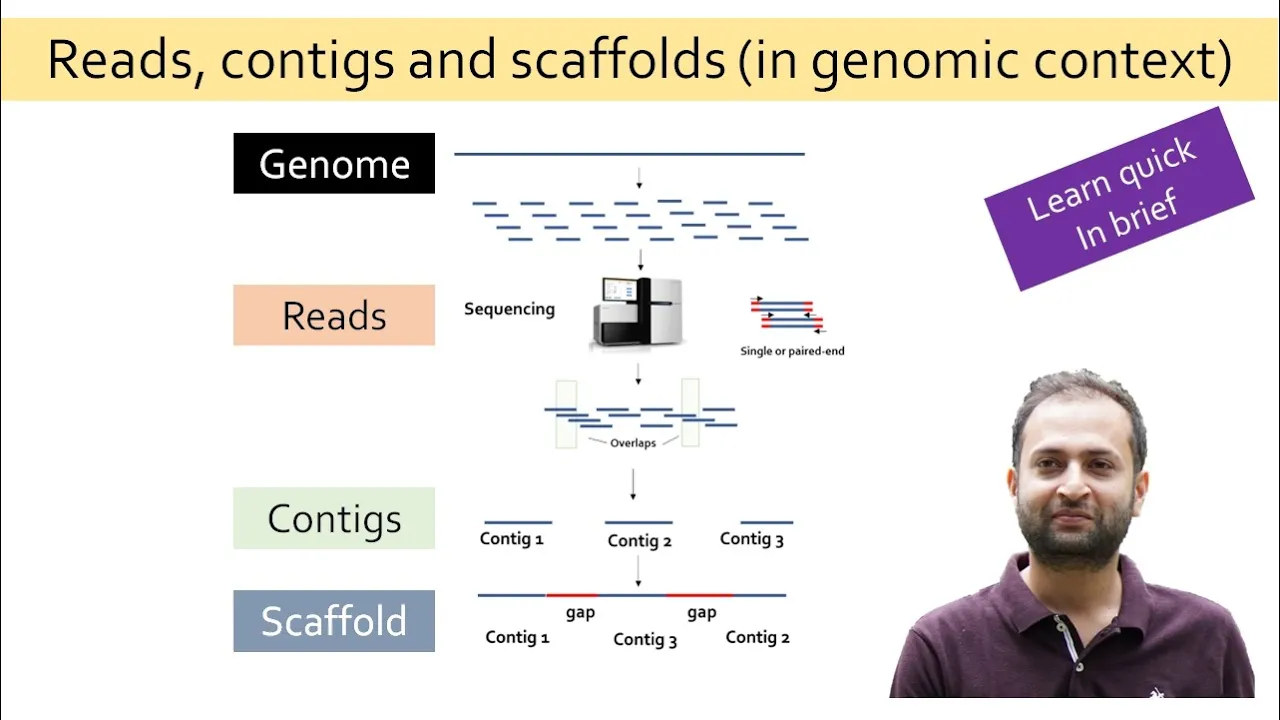
Basic understanding of DNA sequencing workflows, particularly raw read processing, assembly of reads into contigs, and scaffolding.
The conceptual framework of genome binning, which involves grouping assembled contigs into draft genomes based on coverage and composition metrics.
Familiarity with the KBase (Systems Biology Knowledgebase) user interface and the execution of bioinformatics workflows via 'Narratives'.
Methods for evaluating the quality, completeness, and contamination level of MAGs using standardized tools like CheckM or CheckM2.
Taxonomic classification and phylogenetic placement of newly extracted MAGs using reference databases like the Genome Taxonomy Database (GTDB-Tk).
Functional annotation and metabolic reconstruction of the MAGs to predict microbial physiology and ecological roles within their community.
Comparative genomics and pangenome analysis to identify novel genes, metabolic pathways, and evolutionary relationships among related MAGs.
5.7K views96likes54:18Original Release: 2022-12-16
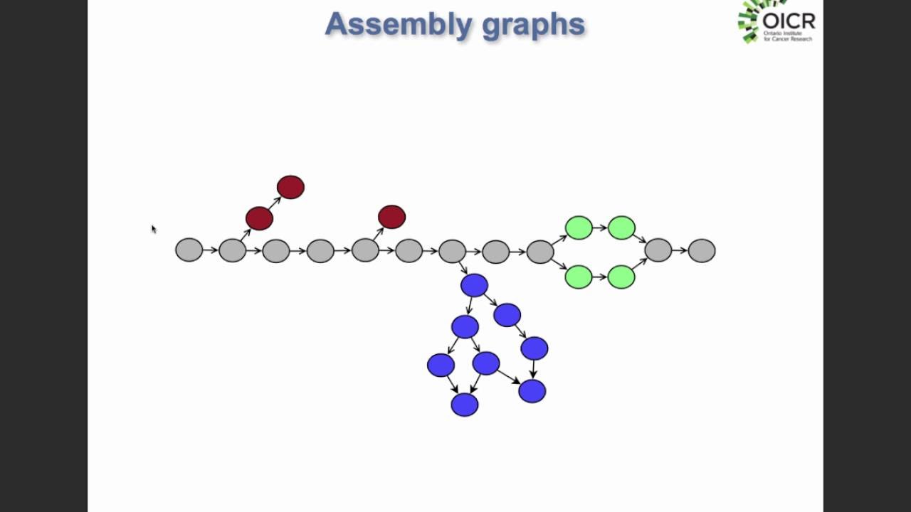
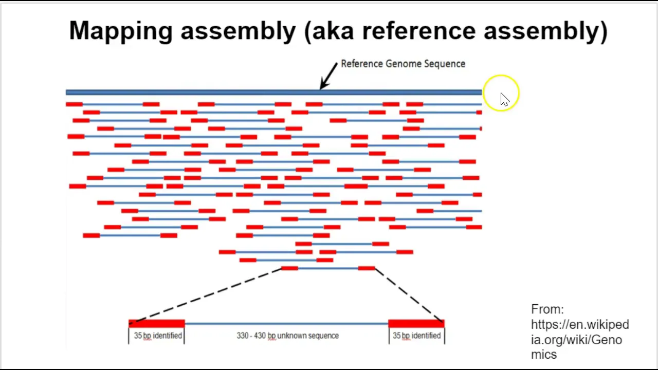
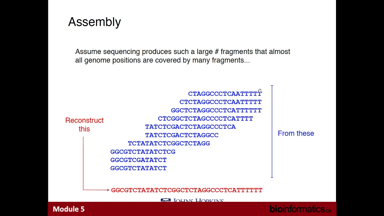
foreign here we have here we have uh the narrative that was used in the paper um and uh so I'm going to take you through the whole thing as Ben mentioned here's the paper um and [Music] um uh there there's uh additionally a published version of this so this is the dynamic narrative or the interactive narrative um but there's also um uh what's called a static narrative or a published narrative version of this uh that you can go and look at and so when you do your own uh research in kbase and eventually you want to publish it you can create this static or published narrative from it and it will exist for you um as a separate thing that's that people can access without even logging into kbase um so but we're going to operate in the uh Dynamic narrative um it has uh basically everything winds up being here and and so since I'm trying to show you how to get through uh building one of these yourself um it makes more sense so the data we're gonna use for this is um uh let me show you the initial input data so we have this compost enrichment from The Joint bioenergy Institute um where they are interested in uh many things but among them um recovering lignocellulose degrading enzymes for biofuel production and so in this compost enrichment they did two enrichments um which they named 37a and 37b and I need to get on my soapbox here for just a second and um explained that how important um doing uh different enrichments and and subjecting your samples to different conditions uh um is absolutely going to give you the best results when you're trying to recover genomes from them uh so literally just take your sample if you have enough and you know put it in 10 or 96 or whatever number of different tubes or you know Falcon tubes or whatever and then change the pH on them change the temperature maybe get creative or if there's some relevant conditions with some um nutrient that they need change that amount and so you're gonna have this leads to two effects which we'll we'll see in this narrative um one is uh certain lineages are going to uh be better have better Fitness for those conditions and their abundance relative abundance will come up in the sample um and so you'll get more reads and so if you do the same amount of sequencing but do it across these different conditions uh these varying enrichments um you're going to get significantly better results because in one of these conditions you're going to have certain lineages come up and another one you're going to have them come up and so you'll get reads from each of those that you wouldn't have gotten otherwise necessarily um and uh so the other Advantage we'll see later is in binning where differential coverage binning is by far and away the best uh way of grouping context from metagenome assembly um and so you'll get a really strong signal if you have you know at least three but you know if you can do you know nine or ten or more um it's really the best way to go and you know it's actually not that hard to do um okay so we're going to start out we have two enrichments in this case 37a and 37b um from compost and we are going to uh start by um I'm going to skip a lot of this sort of description and timing and stuff um you can go back and read it if you want but we're going to start by taking um the reads and importing them and I'm actually I'm going to skip that because I'm going to come back to it at the end um so we've got our reads in kbase as these reads objects um and data in kbase always exists as a structured object um while you can you know export it uh in standard formats like fastq um or import it from standard formats like fastq we store it with with summary information um you can sort of see um how many reads are in the object but it's GC content is the Fred type um what the various quality scores are and so on and so this is very useful for uh operating on in a computational uh fashion um which is how we're gonna need to access all of this so we're going to start by importing them in and then take a look at the quality of these data so for example we have this fastqc app and we can go and we can look at the 37a forward reads for example um and so we're going to look at the per base quality now um there's two things you can do in a narrative to have a sort of more real estate for looking at things you can see this is getting cropped a little bit one is this data pane here and this app pane here well we can go ahead and just collapse those out so we're going to do that here the other thing we could have done is make a new tab with the report so that will open the report in a new tab and give you the full real estate here um so our fastqc report on our our imported reads is well they start out pretty nice but there's really you know maybe it's bleaching or something the tail of these reads is tending to drop in quality the y-axis here is the quality and so this is the distribution of quality scores at that position we can see that the distribution really is falling off uh into poor quality here so what we're going to want to do let me close this up um maybe I'll close this too is we're going to want to trim these reads to keep just the high quality regions and it's gonna um just mean we're operating with with higher quality data um I'll skip the fast QC for the 37b library and so what we're going to do is we're going to use uh in this case trimomatic is a quality trimming tool um and we're going to crop off you know five from the head and and make sure that each read is 140 long so that's usually going to take some off the tail and we can see that um 96.2 percent of the reads survive but in some cases if the entire reverse read is bad then we only get a forward read or conversely with the reverse read and then we're losing 0.3 percent of of all of the pairs um and so if we do that trimming and then look at the fastqc report again for in this case 37a forward we can see that um maybe I will do the separate window um that our tail is now cleaned up quite nicely um okay so what do we do next well um one thing we can do is we can try and figure out which lineages are present in these samples just to get a sense of of um what's the most abundant and where we expect potentially to look for our mags to uh represents in lineage space and so we're going to run this program called Kaiju um and we're going to put in the read libraries and then we're going to select um whether or not we want all taxonomic levels um and then we can pick the reference database and then there's uh something we can do with um whether or not we want to represent the very long tail um you know the population structure of of microbial communities is that there's you know there can be some more abundant ones and where abundant could be even just one percent of the community but you know with a thousands different uh species for example in in a given sample um there's going to be this long low abundance tail and so if we start trying to plot these um relative abundances uh they're gonna you need to start cropping that tail or also you're just going to have a thousand different um uh things showing up for you the other thing that we can do is we can do what's called sub sampling and so Kaiju is going to be running on all these reads and trying to map them to its reference database of um protein sequences and um since we're really targeting the more abundant members of the community um that means we're pretty much going to get the same relative abundance if we look at say 10 percent of all the reads instead of all of them and that's going to save us a lot of time in the run so for example if we look at the job status this Kaiju run only took um an hour and 44 minutes whereas if we'd run on all of the samples that maybe would have been closer to say 10 hours and we get pretty much the same results as as if we had done all of them this is not something that kaijo offers by itself this is something that kbase we added as a way of speeding it up so here we've got our 37a and 37b samples and I'm going to jump to a separate tab um and so we can see that uh the fraction of reads that are classifying or 40 and 50 uh pretty much and so you know what's going on in this uh unclassified fraction um well they may represent novel lineages or they may represent just you know garbage sequence there's just always some weird sequence that shows up um uh and so you know it's not clear what's in the unclassified fraction but we can at least look at the lineage assignments for the classified reads um it may also be that these are reads that are too short to have a uh protein sequence um that matches the reference above some confidence threshold so novel lineage or just simply the read was too short we're talking about alumina paired end reads here that we've now cropped to 140 base pairs so you know a lot of times that doesn't necessarily cross a confident protein so we're getting a lot of proteobacteria we're getting a lot of vectoroidities um and so on at the phylum level um and we can zoom down and and it starts to fragment more you know as you come down so order our family and so on um and so uh we're gonna as you can see this is this is why you want to uh have this tail region um in the report so that you don't see uh it gets longer and longer imagine if we hadn't cropped it at 0.1 percent um and uh you can uh when you go to look at the report um there are in fact um files you can download that will include the uh un Bund uh unbucketed tail so you you will be able to get that information for the download it's just not in a table you just can't see it um in the plot Okay so we've it looks like we've got some um some similar lineages in the more abundant fractions uh in both 37a and 37b um but they are in different relative abundances and especially down here um and so it we're going to go ahead and do a meta genome assembly um so um we have several different metagenome assemblers on kbase one of them is metaspades and so we're going to start with metaspades and we're going to do an assembly um and uh you get a cost report from that assembly and so it'll have a um an accumulation of sequence plot and so on um but let's let's sort of skip that for now because we're going to come back to it so we do a 37a assembly by itself we do a 37b assembly by itself um and then we also since we saw that there were lineages um that were appeared to be related in both 37a and 37b we're going to merge the read libraries as well and this gives us a merged relay read Library which we're going to call 37 a b um and now we're going to assemble the 37 a b as well um here it is it's our input um one thing to note is meta genome assemblies um you know these assemblers will produce you know any joining of reads that they can um but like with lineage abundance you also get this very long tail um where most of the con many many of the contacts I shouldn't necessarily say most of them but often most of them um are very short and so a lot of what we're doing Downstream of this is going to be trying to group these contigs into one lineage process called binning and a lot of the term used there is uh cameras and so very short contigs aren't going to have very strong k-mer signal the other thing is if you're looking for proteins in these contigs um well if you have you know a 500 base pair contig you know maybe I'll perfectly fit a protein in there but a lot of times proteins are longer than that and and so you're gonna really wind up having you know lots and lots of contacts it's going to slow down your analysis and the value of those shorter context is significantly less than the longer ones um especially if you're trying to get at things like genome context and looking at operon structure and so on so what we're going to do here is we're going to cap our or put a floor on our contig length of 2 000 base pairs so that we wind up with um really just sort of the higher quality contigs in our assembly so we run that um and now we have uh the assembly from that and um again we're going to skip the cost report here um because looking at it by itself is is not as meaningful and then we also are going to do assemblies uh with mega hit since we have that and they we're going to do the co-assembly there um we're going to do it with both the meta large where you expect uh uh you have a preset set of parameters for um tuned to a Complex Community we're going to do meta sensitive where it's going to put more work into assembling the um more abundant members um and then we also have idba UD which is a method optimized for uh variable population structure in your community um and the fact is we don't know going in which of these assemblers is going to produce a better result um so we're trying a few of them you may know um which one you prefer or you've done used one or two of them on your data and so you don't necessarily have to go in and use all these assemblers um but this is for sort of the illustration of variation that you get out so now we're going to compare these contigs that we get from each of these assemblers and here's a table that does so so um but we also have an app uh which is very much like cost um but I found cost was missing a few things that I wanted like histograms of the lengths so I added those in this app compare assembled contact distributions um so uh we retained the cost like um cumulative length uh plots and sorted content length plots um and you can see here that the co-assembly with metaspades produces the greatest proportion of long contigs um and as I mentioned uh you know what I'm going to open in a separate tab um as I mentioned before um I wanted to be able to look at the length histograms uh so I created this app um and you can see that um there are more long context even up to 1.4 megabases um in the 37ab metaspades assembly um and these other you know Mega Hit And idba they're they're doing a pretty good job too um but the you can see here the the larger proportion of the distribution is occurring for the 37 a b metaspates context and this isn't necessarily valid in terms of uh metaspades tends to optimize joins um uh with little less support let's say than the the other methods so it's possible that you know we're getting false positive uh joins uh just for the sake of having longer context but maybe it's getting you know because it's doing more joins some of them are true positives as well so um it's like anything in bioinformatics there's a balance between sensitivity and specificity and in this case we're uh going to lean towards uh sensitivity um but sometimes maybe with depending on what you're doing you want more specificity so um okay so now we have our assembled contacts and we're just going to move forward with the co-assembly using metaspates um in this case and we're going to start and um use max bin 2 as one of the binners we have um so with this uh as I mentioned um having variation in your samples uh is very strong signal for banners um which these days all use uh relative abundance as one of the strong signals for trying to group The contigs into one lineage genome or bin so what we're going to do is we're going to take our co-assembled context and then we're going to have the different separate read libraries um as the input so 37a by itself 37b by itself and we're going to produce a Bend contact object as the output um and so uh we run the binner and we get 68 bins and 82 of the contigs are binning you know 18 or not um and so on um but then uh by itself a given Banner is is only so reliable so what we're going to do is we're going to also run metabat which is a binner um that uses uh camera frequencies and relative abundance as well but has a slightly different parameterization for Max bin 2 and it's going to produce its own set of bins in this case 76 um and then we're also going to run concoct and concoct makes 106 bins um but by each each which of them is right well none of them um can we improve on them um I should say none of them are perfectly right uh so can we improve on what they've got by building a consensus and so um I'm sure most of you have heard of uh Jill Banfield and so out of her lab they developed something called dos tool which takes different the input from different binners um in this case our Max bin 2 metabat 2 and concoct bin assignments for these contigs and it takes in the context themselves and then tries to build a consensus set of bins out of the input bins and so if we look at the results um so in this case uh the evaluation of the bins um is done with uh single copy Universal genes and so these are typically ribosomal proteins but there are others uh that are used as well like um RNA polymerase B and so on um gyrase DNA giras and so on where it's a essential Gene uh for microbes but you it if you wind up duplicating it and you have Divergence in it that can kill the cell and become toxic so only one copy is maintained and so um because these are such important genes they can be used um to uh you can make the statement that they are almost always uh present in a single copy in a genome and so you can evaluate the quality of genomes uh without knowing its lineage At All by how many of these single copy Universal genes are present in it and so that's what's being done here is how many of these are present in a given bin so here are the inputs um uh Max bin 2 metabat and concoct and here's the Dos tool bin set and you can't really see but um there are more of the bins that have that are more complete um and it's easier to see with uh this report where you have Max bin 2 metabat 2 concoct and then the Dos tool um where the dark blue here are the bins that are greater than 90 complete by single copy Universal um or single copy Gene is what they're calling it but it's also Universal uh you just more of the bins are more complete and so high quality medium quality and so on um you just have better quality so we're going to take the Dos tool consensus bins as our bin set and that's 40 bins here and now we're going to assess the quality not by just the single copy universals but we can use a tool called checkm um and there's a newer version that's coming out well it's out now but it hasn't fully been released called checkm2 we don't have checkm21 system yet but we will once check M2 is sort of fully released and published um so in the meantime we're going to use checkm and what checkm does is it takes the bin and looks through not just for the single copy Universal genes but it does a phylogenetic placement of the bin genome um into its species tree um and the species tree um allows you to calculate additional genes that are single copy markers for that lineage um so for example um maybe you are talking about the sulfavibrio and if you place a bin into self-vibrio you know that all of the sulfate uh reducing Machinery also is going to be present maybe not a single copy but um there will be collections of genes uh that are um you know essential for that lineage to function and so you can expand the single copy markers into lineage specific or clade specific marker sets and so that's what chechem is doing is it starts by um taking your input Bend context so I you know used the name of the object to sort of capture the history of it and it's too much detail to go into here but we have a system on kbase uh called provenance where you can actually track the data objects and the apps that have been run on them to produce that a given object like this bind contact object um but just for my ability to track it without resorting to looking at the provenance graph um I embed a bunch of information in the name that it's the go assembly for meta Spades and that these are the three binners that went into dos tool to produce the bin context um so uh we're gonna go and and uh run check him you have a choice of either the full species tree or a reduced tree and we're going to save all the plots that Checker makes so we can download so here we have um the checkum plot um so we have all of our bins and they're being scored by how many of the clade specific markers they have um so here you can see there quite a bit more than you know say 40 or 50 there's a very varying number of uh what is considered a single copy Universal Gene um or bacterial Universal or archaeal Universal but you know typically it's on the order of 50. so we're getting more than that here and so we're getting representation of a bunch of the markers for bin 30 but a lot of the others are missing that's what these Grays are um and then for some of these lineages um like bin one for example they're actually quite a few markers that are being found and so you wind up um with the plot having very very fine lines here and sometimes if it's too small it'll actually just be very uh very hard to see the separation anyway so if we go down to the like this bin 20 for example um so if we go down to the bottom here is there's the uh um the key to this plot and that is um green means that there's a single copy of that clade specific marker gray is missing and then that we have this additional uh two colors blues and and orange Reds and that is meant to indicate uh in the case of uh blue when there's more than one copy of that Gene family showing up in the genome and if it winds up being uh um close to the or if the multiple copies wind up being close to one another um then you can say it's probably a paralysis expansion of that Gene family in that lineage um it still may represent strain variants genomes that are being mixed um but it's hard to distinguish that from um a paralysis expansion in the lineage that's legitimate and so those are these they're light blue in this say bin 47.
um contamination is when you have more than one copy but the two sequences are distal to one another and those are more likely contamination in this case not contamination of the sample but the bins themselves have had their contigs mixed um and and you know maybe it's correct and maybe it's not but um overall you're you can see that um hmm why can I not scroll there we go um um that the best of the bins are here at the bottom of this plot in the and the worst quality ones are here at the top um we also offer a table where you can look at the completeness and contamination um of each of these bins numerically um and again you know one has to take these numbers with a grain of salt because if it's a Well studied lineage then yeah maybe the clade specific markers are valid um but then you have other lineages like peteskey bacteria where um it's the knowledge of what are the specific markers is is less well in hand and so it may wind up with a completeness score that's less than say 90 even if it's a complete genome so um these are you know these are approximate guided lines um so what we're going to do uh following this is we're going to filter out the lower quality bins and we're going to because we have so many really high quality bins from this um again enrichments are a good way to go um we have we are able to uh Threshold at 95 completeness and two percent contamination and so we're going to do that to find the really really best quality ones and um we've made a variation of the Checker map where we um filter the bins uh for you in this app and so it'll produce a bin contigs object as its output um that is just the high quality 95.2 and here I need to make a quick statement and that is um what we're calling high quality here is based dust on the checkum completeness and contamination scores um metagenome assembled genomes from short read sequences like we have here um alumina for example um often have difficulty assembling uh ribosomal RNA genes um this is because uh they're often present in more than one copy in a genome and therefore the assemblers get confused um and don't wind up being able to span repeats this is also true for you know longer transposons where there can be multiple copies that are identical or virtually identical in the sequence and so this breaks assemblers abilities to join um join those shorter contacts as they're doing the assembly so here we wind up filtering out those short ones um sorry it still reports all of them um but if you look at the table you'll see in red here uh what was below our thresholds um so you know here this bin 4 actually is pretty good quality but it's below our very strict 95 2 percent threshold and so it gets filtered out from that bin contig um and then we're also going to do uh one at 90 and 5 uh 90 completeness and five percent contamination um just to have capture those that are sort of in the middle and so we'll have a set of Bin contacts there so now what we need to do is everything is stored as a binned contig object but what we need to do is pull out each of those as a separate assembly representing um that lineage and so we're going to run this extract bins as assemblies uh method and we're going to run it say in this case on the 90 completeness five percent high quality fraction um and it's going to pull those out and it's going to produce assembly objects for us um and it will also create what's called an assembly set and it's this is a nice object uh to have because um now instead of having to add each of these assemblies um at once uh separately to apps that are Downstream we can now just give it the assembly set that that holds them inside and that means that it's much easier to run these apps so for example after we have these assemblies well now we need Gene calls on them so we can run uh annotate multiple microbial assemblies this rast app um but instead of having to input each one of these assemblies one by one which you could do if you had a certain subset that you wanted to work with we can instead give it this 95 assembly set as its input and it will produce a genome set um as as its output so it'll produce genomes which are assemblies plus Gene calls um plus annotation functional annotation and um Additionally the genome set that we can use as a single object input for other apps so now we're going to run we're going to try and get a better handle on what the lineages are for these um mags so now that we've pulled them out of the bin contigs and we've decided that these are going to be um you know these are the high quality ones we're gonna you know go forward with analyzing them like they were similar to isolate genomes we're going to start calling them mags now because they have Gene calls to them they really do look and can be operated on like um Regular uh isolate genomes um so now we're going to use this method called gttbtk so gttb is a um a whole genome-based alternative for uh taxonomic classification and so what the hugenholtz group and um has done is they have taken all of the um mostly high but some medium quality genomes isolates and Mags from and CBI and built uh whole genome species trees using the single copy Universal markers uh for um tree building and they can then um use that to go and place new genomes new mags into uh into that taxonomic classification scheme and so that's what gttbtk does it it does two things it one it runs fast a and I for a quick assignment but then it also does a phylogenetic placement in the tree using p Placer and so you'll wind up being able to uh for those genomes that can be classified uh um you'll get some classification in the gttb uh taxonomic space in this case bin three is able to be classified to this genus but not to a species um whereas others at least not on this first page um here um Yuki bin 37 winds up actually being within the uh similarity thresholds to be put into this species classification so you'll get a different range of it some of them will be closer uh down to the species level and others will be just say to the family level or so on um so now we have these uh and um we've updated the genome object to contain this taxonomic classification um now we also want to look at these within the species tree context and so we're going to take our bins and we're going to put them into a species tree against refseq genomes using the species this insert set of genomes into species treat app um now the species Tree app has a tendency to uh just find the closest genomes and so you can wind up with a situation where lots of genomes are going to be found for certain lineages um but then others uh so for example this bin 43 here is finding lots of these lineages they're just well represented and close to this bin in refseq whereas some of these other bins are not not finding the closest relatives and so what we need to do is split up our bins into different clades so that we don't wind up having you know examples like bin 43 sort of dominating which um species show up um in the species tree so we're going to split them up into clades and we're going to do this manually using this build genome set where we specify well those are missing um specify that clay day is going to be bins 3 42 57 and 59 which is what is supposed to be showing up here and that's based on well I'm not oh here we go yes 59 3 57 42. so that's clay day and we're going to do that um for clades a through k so this is just by eye looking at the species tree that was generated with that first run and then we're gonna go and insert each of those clades separately into the species tree to find the proximal genomes so here's all the build build genome set runs um until we have K and then we're going to insert um in this case clade a uh into the species tree and we're just gonna we're gonna add 20 refseq genomes into that tree and it's going to give us um more proximals um refseq genomes here's clade B and so on so anyway this is a a way of sort of allowing us to figure out what are the close relatives um to our bids and potentially we want to include them in Downstream analyzes of say function or pen genome analysis or something like that um that type of Downstream comparative genomics um uh we're not going to have time to discuss today but um early in in 2023 um I'll do another webinar where we go through that that whole process so um we're gonna go and finish inserting our clades into the species tree and finding all the refseq proximal genomes um or a bunch of apps runs here um additionally maybe we don't want just the proximal refseq genomes but we want to have a sort of bigger picture phylogenetic context and so we can build a species tree where we have genomes that represent a given phylum that are sort of forced to be in the tree and so that this build microbial species Tree app allows you to do that um so we have our uh um mags with we're gonna use as a genetic skeleton um the bacteria since we know we don't really have any archaea in this set of mags but you could use bacteria plus archaea isolates mags and sags you could use just bacteria isolates and so on here we're going to do sort of all bacteria mags and sags and we're going to have our phylum skeleton species tree and now we can look at um the bins in this phylogenetic you know super context where the phylum context I should say um and I'm going to zoom in a bit on this so uh here we can see our these bins are showing up in Alpha proteobacteria um these bins are showing up in Vero mic varicomicrobia and so on um here's our bacteroidity sclerobi [Music] um so that's another sort of phylogenetic app we can use and now we want to look at the functional classification of these mags and we have several different tools for this as well um so you know we ran rest and that can give us seed classification and there's tools for looking at the functional profile of seed you can run uh Cog or pfam or tiger fams annotations on these genomes and you can look at uh the functional profile of those domain classifications um here I'm going to talk about a little bit about the dram uh functional distillation app um where we put in our assembly set um and we're going to get uh genome annotations using dram out of that um and additionally uh tram provides this really nice table um sorry these are all the created objects uh here at the top um Can collapse that um and instead look at the dram report and so here we have each of the bins as rows and then these different dram functional categories as columns and so you can have electron transport chain classification there's these different glycolysis modules and so on and then additionally um for metabolisms Dram offers KZ classifications uh um nitrogen metabolism and so on so that's one route towards functional classification of your bins um We additionally can use direct Hammer profiling we have several different Suites of Gene families available and are expanding that those different sets right here I'm explaining I'll tell you about the Casey family since this is a particular interest for this study the dbcan group has taken the KZ families and built hmms out of them and so we can run our bins through that and we can get the GH ones um gh2s and so on and one nice thing about the hammer app is we can when we configure it you know we put in our genome set and we can pick different families but we can actually specify particular families like say GH4 um and then we can choose to save feature sets uh for explicitly requested models you can save it to all all models but then you end up with a ton of feature sets one per Gene family so in this case we're going to save Only Hits or we could save Only Hits to explicitly requested models like so for example like I said GH4 or something and that would produce a feature set that we could then use in subsequent analysis again I don't have time to go into that today um one of the collections of Gene families we offer uh hmms we offer is called micro trait and we can use microtrate in this uh summarized genome set app um where uh to give a sort of functional summary classification for each of these mags and then Additionally the summarized genome set can run check them for you it can add this microtrade bio elements you can choose to um show just the newest genome version as you've updated it over and over and so on um and you can use the there's different parameters for checkuments on that you can include so um since I'm tight on time let me just keep going forward here and we have our bins and we have these sort of uh summaries of the functional categories and we can uh see that bin 3 doesn't seem to have any of the nitrogen fixation genes but for oxygen tolerance and utilization we have these genes families showing up um there's cisen and so on uh Bin 11 is showing up uh you know bringing in Sox B socks why and so on so we have the ability in the summarized genome set app to have the genome the mag it's a functional summary and what genes are present in it um and this is downloadable as a table too so you don't have to just eyeball um rollover the taxonomy of it it's checking completeness it's contamination how many contigs are in the mag the genome size if you sum the sequence of those contigs it's n50 it's GC how many coding sequences there are cds's how many trnas are present and this is as I mentioned uh a lot of mags don't wind up getting the ribosomal rnas assembled because of the fact that they're repeats and this is a a shorter read technology there are long read Technologies coming online for metagenome assembly that resolve this problem and so it's really probably best to use a combination of the two but we are getting crispr arrays and so on so there's this summary does show up and in fact sometimes you do get a 16s here and so it's still not going to meet the me mag threshold for uh you know isolate level quality um but bin 37 appears too um and so on so um so you can use the summarize genome set to sort of uh have a look at everything that's coming out of your mag recovery um so uh we'll be uh like I said in early 2023 uh be doing a comparative um uh metagenomics and and mag analysis uh tutorial um there's a bunch of reference literature here um and let me go back up to the top since I'm just about out of time this narrative as you can see it's chock full of data already um and you may want to be going through this analysis with your own data um and this is you know going to be in the way and all these app cells are already here and so what we've done is produced a blank narrative or a reset narrative or a template where the data has been removed the app runs have been removed um and so what you want to do is cut goat go to that narrative um and then copy it maybe you want to wait a little bit so we don't all wind up doing it at the same time and um because this is as hard for the system you go to this template narrative click on narratives here at the top well it's a little slow anyway then you would click on copy this narrative um give it you know a new name like um my metagenome narrative um version one copy it because you're not going to be able to edit this template one you're you're going to want to make a copy of it so that you can it's your copy and you can work on it and it's your private narrative and so on so now I'm going to open that up and then this is the one you're going to want to import your data to um and all of that so uh we're out of time and so I'm going to very quickly see if there are any questions that haven't been addressed uh so things begin to Dylan and the whole k-based team for all the work that went into this paper and this uh the narratives associated with it and we hope to see you all next year on more of these uh k-based webinars and of course we hope to see you on the system and I look forward to all the papers that you will have coming out using those pipeline so okay take it easy everyone and we'll post this recording up uh tomorrow or so on our YouTube page so thanks again thanks for watching this webinar for more webinars and tutorials subscribe to our YouTube channel you can see announcements for upcoming webinars and recordings for previous webinars on our website at kbase.us learn let us know in the comments what content you'd like to see in future webinars be sure to follow us on Twitter At Doe kbase and if you have questions or encounter an error when using kbase please contact the help desk
Up Next

51:10
Marine Natural Products: From Sea to Pharmacy | Ocean Science Lecture
@uctv
24.4K views•2019-09-03
50:12
Bacterial Communication: Quorum Sensing and Biofilm Formation Explained
@JHUAAP
12.6K views•2011-06-28

5:35
Enteric Nervous System Explained: The Gut's Brain | Neurobiology Lecture
@alumniu6029
438 views•2018-09-12
7:08
Bacteriophages: Earth's Deadliest Killers and Future Antibiotics
@kurzgesagt
34.6M views•2018-05-13
Related Study Plans & Knowledge Roadmaps
Structured learning paths in Biology
biology
RNAi: Biogenesis, RISC & Gene Silencing
01Molecular Biology Foundations: DNA to Protein
02Introduction to RNA Interference (RNAi)
03Molecular Biogenesis of miRNA and siRNA
+ 2 more learning modules
10h5 modules
Explore Roadmap
biology
Mycorrhizae: Signaling, Biophysics & Ecology
01Foundations of Mycorrhizal Symbiosis
02Molecular Signaling and Root Colonization
03Biophysics and Bioenergetics of Nutrient Exchange
+ 1 more learning modules
11h4 modules
Explore Roadmap
biology
Circadian Clocks: TTFL, SCN & Periphery
01Foundations of Molecular Biology & Gene Expression
02Introduction to Chronobiology and Actograms
03The Core TTFL: Molecular Architecture of the Clock
+ 3 more learning modules
14h6 modules
Explore Roadmap
biology
Population Genetics: Math, Drift & Selection
01Genetic & Probability Foundations
02The Hardy-Weinberg Principle and Baseline Models
03Mathematical Modeling of Natural Selection
+ 3 more learning modules
18h6 modules
Explore Roadmap