

























![Regularization in ML explained simply | Lasso (L1) and Ridge (L2) | Foundations for ML [Lecture 27]](https://i.ytimg.com/vi/VNrdslReSZU/maxresdefault.jpg)


Gradient descent is an optimization algorithm that minimizes the mean squared error (MSE) cost function by iteratively adjusting parameters (m and b) using partial derivatives and a learning rate, allowing the algorithm to find the best-fit line for linear regression through a series of small steps toward the global minima.
Gradient Descent & Cost Function Tutorial for Linear Regression Python
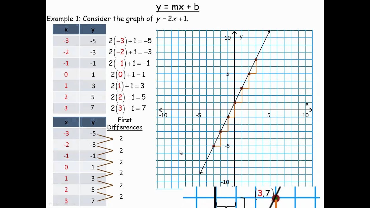
Added:Basic algebraic concept of a linear equation (y = mx + b) and the interpretation of slope and intercept.
Fundamental Python programming, including writing functions, loops, and working with basic data structures.
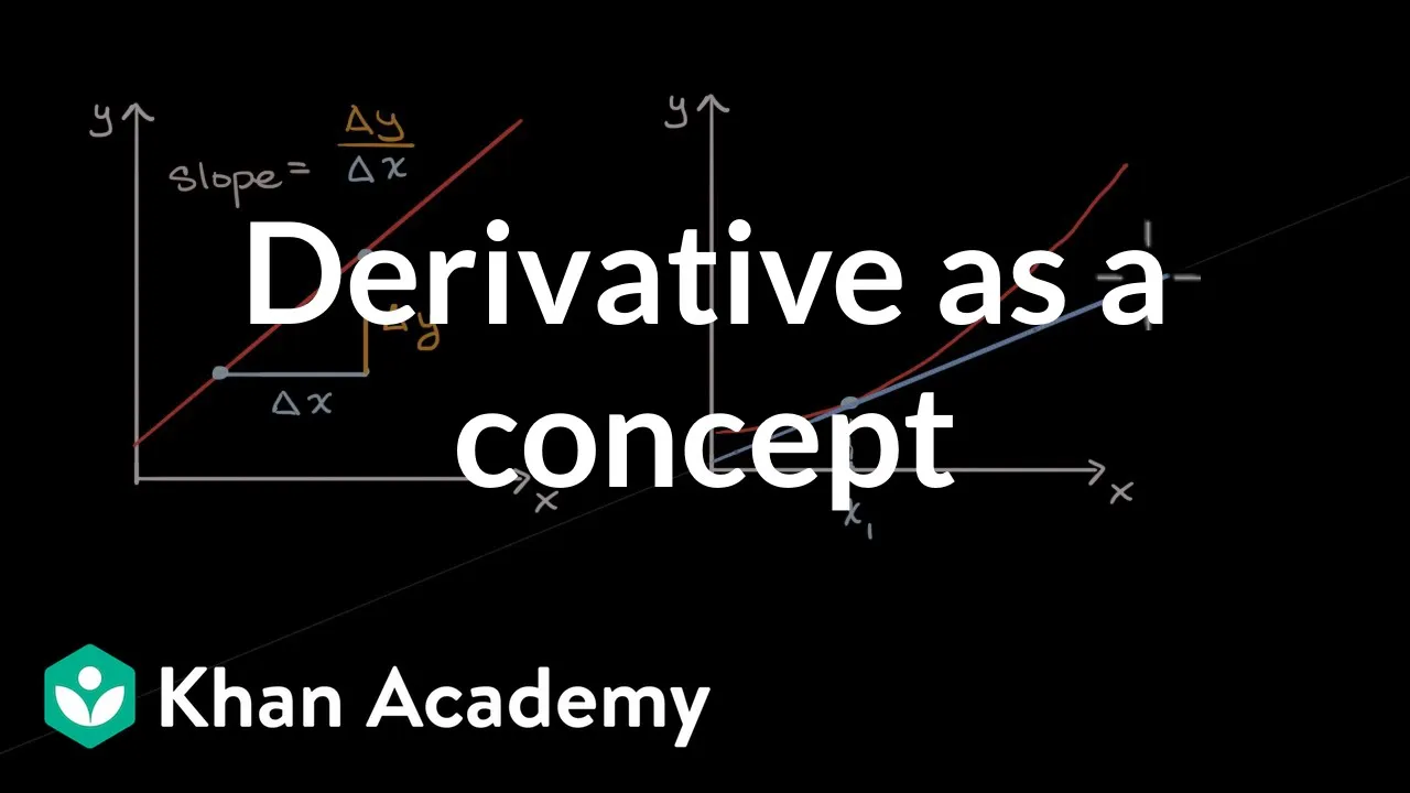
Introductory calculus concepts, specifically derivatives as rates of change and how they represent the slope of a curve.
Understanding of basic statistical metrics, particularly how errors or residuals are calculated between predicted and actual values.
Multiple Linear Regression and the use of matrix calculus and linear algebra to handle multiple predictor variables.
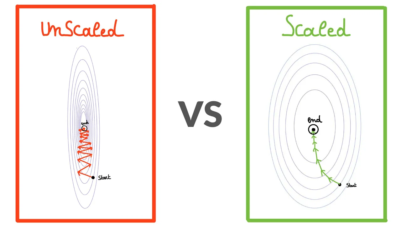
Feature Scaling and Normalization techniques (such as Standardization or MinMax Scaling) to ensure faster convergence of gradient descent.
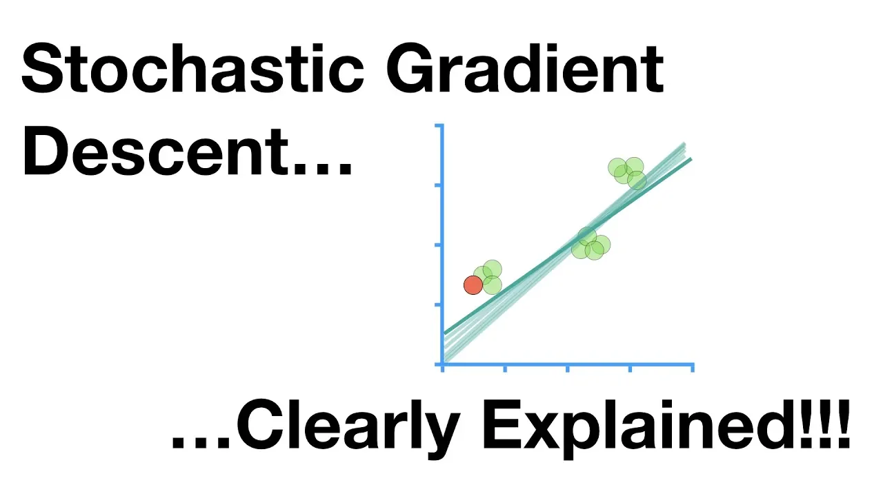
Advanced optimization algorithms, such as Stochastic Gradient Descent (SGD), Mini-batch Gradient Descent, and the Adam optimizer.
Regularization methods like Ridge (L2) and Lasso (L1) regression to prevent overfitting and improve model generalization.
Hyperparameter tuning strategies, specifically focusing on diagnostic tools to identify learning rates that are too high or too low.
805.9K views11.5Klikes28:25Original Release: 2018-07-22
mean square error, cost function, gradient descent and learning rate.
These are some of the important concepts in machine learning. And that's what we are going to cover today. At the end of this tutorial, we would have written a Python program to implement gradient descent. Now, when you start going through machine learning tutorials, the thing that you inevitably come across is mathematical equations. And by looking at them, the first thought that jumps into your mind is, "Oh my god, I suck at math. I used to get four out of 50 in my math test. How am I going to deal with this? Let's not worry too much about it.
We can take one step at a time and the things won't seem that much hard.
Also, you won't be implementing gradient descent when uh solving the actual machine learning problem. But the reason we are doing this exercise today is that you should know some of the internals so that while using the skarn library, you know what's going on and you can use the libraries in a better way. With that, let's get started. During our linear algebra class in our school days, what we used to have was this equation and x as an input. And we used to compute the value of y where the way you derive 9 is by multiplying this three with two which will be six + 3 and that's how you come up with nine.
In case of machine learning however you have observations or training data set which is your input and output using that you try to derive an equation also known as prediction function. so that you can use this equation to predict future values of x.
In case of our problem of predicting home prices, we saw in the initial uh linear regression tutorials that we have area and price and using that we came up with this equation. Now if you don't know uh this equation quite well, you look at my Jupiter notebook and in that notebook you'll see that I have this coefficient and intercept. Okay, so that's what I have put it here. So here I have the home prices in Monro Township and I have plotted these on this chart and what we are going to look at is how can you derive this equation given this input and output. Okay. So our goal is to derive this equation. That equation is nothing but this blue line which is the best fit line uh going through all these data points. Right now these data points are scattered. So it's not possible to draw the perfect line but you try to draw a line which which is kind of a best fit. All right. But the problem here is you might have so many lines right that can potentially go through these data points. My data set set is very simple here. If you have uh like very heavy data set and if it's it's like scattered all over the place then drawing these lines becomes even more difficult. So how do you know which of these lines is the best fit line?
Okay, so that's the problem that we are going to solve today. So one way is you draw any random line. Then from your actual data point, you calculate the error between that data point and the data point predicted by your line. Okay?
So call it a delta. You collect all these deltas and square them. The reason you want to square them is these deltas could be negative also and if you don't square them and just add them then the results might be skewed.
After that you sum them up and divide it by n. So n here is five. It is number of data points that you have available.
The result is called mean square error.
Okay. And mean square error is nothing but your actual data point minus the predicted data point. You square it, sum them up and then divide by n. This mean square error is also called a cost function. There are different type of cost function as well but mean square error is the most popular one. And here y predicted is replaced by mx + b because you know that y is equal to mx + b. So that's the equation for mean square error. Now we initially saw that there are so many different lines that you can draw. Uh you're not going to try every permutation and combination of M and B because that is uh very inefficient. You want to take some efficient approach where in very less iteration you can reach your answer.
Okay. And gradient descent is that algorithm that helps you find the best fit line in uh very less number of iteration or in a very efficient way.
Okay. So we are going to look at how gradient descent works. Now for that I have plotted MB against the mean square error or a cost function. Uh so here I have drawn different values of m and here there are different values of p which is your intercept and for every value of m and b you will find some cost. So if you keep on plotting those points here and if you create a plane out of it it will look like this. It will be like a ball.
And what you want to do is you want to start with some value of m and b. People usually start with zero. So here you can see this point has m as zero and b as zero. And from that point you calculate the cost. So let's say the cost is 1,000.
Then you reduce the value of m and b by some amount. And we'll see what that amount is later on. So you take kind of like a mini step. You come here and you will see that the error is now reduced to somewhere around 900 something like that. And then again you reduce it by taking one more step. You keep on taking these steps until you reach this point which is your minima. Here the error is minimum and once you reach that you have found your answer because you will use that m and b uh in your prediction function.
I have plotted these different lines and these different lines will have different values of m and b. Let's say this orange has m1 b1. So that m1 b1 will be here somewhere. Blue line will have m2 b2. M2B2 will be this red dot.
Then red line will have M3 B3. So M3B3 will be somewhere here on this plot. So you can have like so many numerous lines which can create this uh plot. Now we just said that you will take this baby step but how exactly you do it cuz visually it sounds easy but mathematically when you give this task to your computer uh you have to come up with some concrete approach. All right.
So we'll look into that. But here is a nice visualization of uh how you can uh reduce your M andb and reach uh the best fit line. All right. So let's look at how you're going to take those baby steps. So I have these two charts. Uh if you look at this 3D plot from this direction, what you will see is a chart of B against cost.
And that will be this curvature.
Similarly, if you look at this chart from this direction, the chart will look something like this. And in both the cases, you are starting at this point which is this star and then taking these many steps and trying to reach this minimum point which is this red dot.
Now, how do you take these steps? Right? So one approach is let's say you take fixed size steps.
So here if you plot this against B I'm taking fixed size steps on B. But the problem that it can create is by taking these steps I might miss the global minima.
Okay, I might just miss it and my gradient descent will never converge it from this point it will just start going up and up and I don't know where is my minima. All right, so this approach is not going to work. What can work is if you take steps like this. So here in each step I'm following the curvature of my chart and also as I reach near to my red point you can see that the step size is reducing. You see like this arrow is bigger and these arrows are getting smaller and smaller. If I do something like this then I can reach this minima. Now how do I do that? So at each point you need to calculate the slope.
Okay. So for example at this point the slope will be this. This is a tangent at the curvature and at this point here my slope will be this.
Once I have a slope I know which direction I need to go in. For example if you look at this green line and if I'm at this blue dot I know that I need to go in this direction.
And then there is something called a learning rate which you can use in conjunction with this slope here to take that step and reach the next point. Now we have to get into calculus a little bit because calculus allows you to figure out these baby steps. And when we are talking about these slopes, really this slope is nothing but a derivative of B with respect to this cost function.
Okay, if you want to go in details, I recommend this channel three blue one brown. This guy is very good in explaining mathematical concept uh using a nice visualization. So you will really uh find it uh very useful and pleasing.
But if you don't want to go in details then in this tutorial I'll just quickly walk over some of the basic concepts.
Okay, let's look at what is derivative.
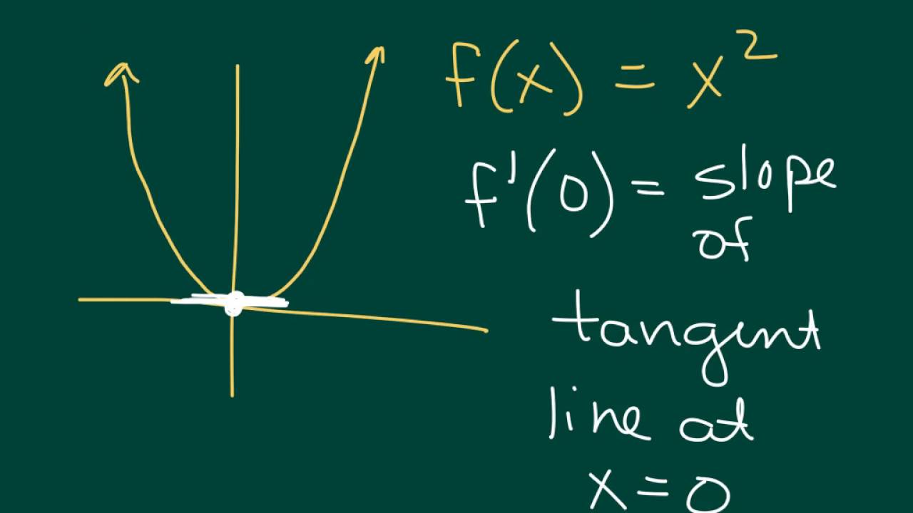
So derivatives is all about slope. I'm on this uh website called math is fun and these guys have explained it really well. So slope is nothing but a change in y divided by change in x. Okay. So if you have a line like this and if you want to calculate slope between the two points here it is 24 by 15. But what if you want to calculate the slope at a particular point right? Like in our case if you remember here we want to calculate the slope at a particular point. Same thing here right?
So that slope will be nothing but a small change in y divide by a small change in x. All right.
We'll say uh as x shrinks to zero and y shrinks to zero that's when you get more accurate slope. Okay. So for the equation like x² that slope will be 2x.
Okay. This is again called a derivative.
derivative is mentioned by this notation d by dx and the derivative of x² is 2x.
So for example for this chart the slope here is 4 because this is x² and and the value here for the slope will be four.
Okay. Now let's look at what is partial derivative. When you have an equation like this where you have your function depending on two variables x and y what you try to do is you calculate a partial derivative of x. In that case you keep the y0. So here fx is nothing but a partial derivative of x² with respect to x. Okay. Similarly, when you want to calculate the partial derivative of this function with respect to y, what you do is you keep x0 and then you uh calculate the derivative of y. All right? And general rule here is let's say if you have y cube, right? Like how did you come up with 3 y^2? Like you put three here in front of y and then you subtract one from 3. So that's how you get 3 y square.
Okay. So those are like some of the basic concept of uh derivative and partial derivatives. Again if you want to go in detail just follow a three blue one brown YouTube channel and that guy is like really good in explaining these concepts in detail. Okay. Okay. So just to revise the concept, the derivative of this function will be 3x² and this is the notation for your derivative.
The derivative of functions which has dependency on two variables. It will be a partial derivative and the partial derivative of this function with respect to x will be this and with respect to y will be 2 y. And this is how you mention your derivative. This is the notation that you use, right? It's sort of like looks like a D, but it's not like it's like a curved D. So now going back to our problem of the line, right? So here we want to find the partial derivative of B and then for the other chart we want to find the partial derivative of M. Okay, so how do you find that? So this is your mean square error function and the partial derivative of m will be this and partial derivative of b will be this.
Now I'm not going to go in detail about how we came about this. Again you can follow other resources but you can just accept this equation. It's sort of like a rule you know it's like uh why earth rotates around the sun or why humans have two eyes. Well it's just a law of nature. But if you want to go in detail on how we derived this then you can follow some other resources. But one hint I can give you is see this thing has a square. So generally for a derivative you put two here. So 2 cm here and this becomes 2 minus one which is one which we don't uh show here. All right. And then once you have partial derivative what you are having is a direction. So partial derivatives gives you a slope. And then once you have direction now you need to take a step.
So for the step you use something called learning rate. All right. So you have initial value of m and then you subtract uh this much your learning rate into slope. So for example you are here on this chart. This is your b1 value. To come up with this B2 value, you will subtract learning rate multiplied by the partial derivative which is nothing but a slope here.
Now let's write Python code to implement gradient descent. I'm going to use Pycharm today instead of Jupyter notebook because I'm planning to use some of the debugging features.
Pycharm's community edition is freely available to download from Jet Brains website. The problem we are solving here is we have a value of x and y vectors and we want to derive uh the best fit line or an equation using m and b. So you have x x and y and you want to come up with correct value of m and b. All right. So that's our objective here. I'm going to use a numpy array instead of simple python list because uh matrix multiplication is very convenient with this and also numpy array tends to be more faster than simple python list.
So the first thing we are going to do is start with some value of m current and b current. All right. So again to revise the theory uh you start with some value of m and b and then you take these baby steps to reach to a global minima. So as you can see in the chart we started with m and b values as being zero and then we took these steps one by one to reach the global minima.
Another thing you know need to do is define the number of iterations.
You have to define how many baby steps you're going to do. I'm going to start with 1,000 and then I will fine-tune it.
Okay, again all of this is pretty much like a trial and error. I will start with some parameters and I will see how my algorithm behaves and then I will fine-tune them. All right. So let's run a for loop. simple for loop which just iterates these many iterations.
And at each step what you do is first thing is you calculate the predicted value of Y. All right. So Y predicted is nothing but M current into X + B current. All right. Pretty straightforward. Y is equal to MX + B.
And for the assumptions that you have for M and B, you are calculating Y, which is Y predicted. Next step is to calculate M derivative and B derivative. So M derivative, I'm going to call it MD.
And the equation is 2 by N. All right.
Now, what is N? N is the length of these data points.
I'm assuming X and Y's length is same.
If it is not the case, then you can add necessary validation and throw an error.
All right. Uh so M's derivative is -2 by n multiplied by sum of something. What is that sum? Sum is uh x multiplied by y - y predicted. Okay. So y - y predicted and b's derivatives equation is same except the fact that it doesn't have this x multiplication.
Once you have that you're going to adjust your m current as shown in the equation.
uh your next m will be your current m minus learning rate into uh m derivative. So we have m derivative but we need learning rate. Okay. So I'm going to define learning rate now.
Okay. Again this is a parameter that you have to start with some value. So I'm going to start with 0 1. People generally start with 001 and then they gradually improve it. You can remove zeros. You can you can use like five whatever. This is like trial and error. You see how your algorithm behaves and then you tweak those parameters.
Similarly for B the equation is your value of B is B minus learning rate into your uh partial derivative and then at each iteration I will print their values.
Let me print iteration also so that I know what's going on at each iteration.
Okay.
All right. So, looks like my code is good enough and I can just run it. So right click and run it.
Okay. So let's see what happened.
So you can see that we started with some value of M and B and now in the end we are at 2.44 and 1.38.
Okay. Now if you want to know how well you are doing you need to print cost at each iteration you should be reducing your cost right so if you remember the 3D diagram at each step you should be reducing your cost sometimes if you don't write your program well and if you start increasing the cost then you are never going to find the answer so let's print cost so what is our cost is equal to if you check the equation it is 1 divid by n multiplied by sum of something and that something is all the data point differences between y and y predicted and their squared. So we need a list here and the value in each of the the list element is this.
you will run a for loop on for value in y - y predicted and I'm using a list comprehension here and for each of these values you want to take their square and this is to deal with the negative values after that I will print the cost at each iteration and when I run this.
I can now track down the cost. You can see the cost is reducing in each of these steps.
Now, how do I know when I need to stop?
So, I can keep on increasing my iterations.
And you can see that I'm getting closer and closer to my expected m and b value, which is 2 and three.
You can also manipulate your learning rate. So what I usually like to do is first I will keep the iterations less. I will start with some learning rate and I will see if I'm reducing the cost on each iterations. So here with this learning rate I can see that I'm reducing my cost.
Okay. So I can maybe take even a bigger step. So I will do probably zero and let's see what happens with that.
Now here yes. So uh with that also I'm reducing my cost. So I think this is fine. Let me try one more bigger step which is this.
Now you can see that I started increasing my cost. So this learning rate is too big. I am crossing my global minima and I am shooting in the other direction. So I have to be between 01 and.1.
So how about 09 there also I'm increasing. So maybe 08.
Okay, that looks good. Here I'm reducing. All right, so I I will stick with this learning rate and increase my iterations to let's say 10,000.
You can see that now I reached my optimum value. The expected value of M was 2 and B was three. So which is almost near to three. And you can see the cost is very minute. This is how you can approach your gradient descent algorithm and stop whenever you reach some threshold of cost or even you can compare the cost between different iteration and you can find out see the the property of this uh curvature is that once you reach the global minima your cost will kind of stay the same.
Okay. if you're using the correct learning rate. So here you see all in all these iteration your cost is almost remaining constant. So you can use uh comp floating point comparison and just compare to cost and stop whenever your cost is uh not reducing too much.
I also have a visual representation of how my uh MNB is moving towards the best fit line. So we started here and then we gradually we were moving closer to those points. The those red points are not quite visible but they are here here and you can see that gradually I am reaching more and more closer towards those points. So you can use this Jupyter notebook for uh visualization purpose.
And now we'll move into our exercise section. So the problem that you have to solve today is you are given the mathematic and computer science test scores for all these students and you have to find out the correlation between the math score and computer science score. So in summary, B is your X and computer science score which is column C uh as your Y. Using this uh you will find a value of M and B by applying gradient descent algorithm. And what you have to do is you have to compare the cost between each iteration and when it is within certain threshold. And to compare the threshold we are going to use a math do is close function and use a tolerance of 1 e to minus20.
Okay. So if your two cost are in this range then you have to stop your for loop and you have to tell me how many iteration you need to figure out the value of m and b.
Up Next
9:54
Random Forests Explained: Build, Use & Evaluate ML Models
@statquest
1.4M views•2018-02-05

57:48
Secure Multiparty Computation (MPC): Foundations & Challenges
@SimonsInstitute
7.3K views•2015-05-28

13:03
Bypassing Tor Censorship: Bridges and Pluggable Transport Guide
@Coding_ForEveryone
397 views•2024-06-11

18:41
Neural Networks Explained: Math, Layers, and Learning Fundamentals
@3blue1brown
21.9M views•2017-10-05
Related Study Plans & Knowledge Roadmaps
Structured learning paths in Artificial Intelligence
artificial-intelligence
Aligning LLMs: DPO, TRL & Custom Datasets
01Foundations of Python & Machine Learning
02Transformers and Large Language Models (LLMs)
03Aligning LLMs: SFT and RLHF
+ 3 more learning modules
24h6 modules
Explore Roadmap
artificial-intelligence
Federated Learning: PyTorch, Flower & Privacy
01Python & Machine Learning Foundations
02Deep Learning Basics with PyTorch
03Introduction to Federated Learning
+ 2 more learning modules
35h5 modules
Explore Roadmap
artificial-intelligence
Securing LLMs: Guardrails AI & NeMo Gateway
01Introduction to LLMs, Python, and APIs
02Understanding LLM Vulnerabilities & Threats
03Defending LLMs with Guardrails AI
+ 2 more learning modules
15h5 modules
Explore Roadmap
artificial-intelligence
Building Recommenders: Two-Tower & Vector DBs
01Foundations of Python & Machine Learning Basics
02Introduction to Recommender Systems
03Deep Learning & Representation Learning
+ 3 more learning modules
75h6 modules
Explore Roadmap