











Spectral clustering is a powerful machine learning technique that partitions data into clusters by leveraging the eigenvalues and eigenvectors of a graph Laplacian matrix, offering significant advantages over traditional methods like k-means and EM: it makes no assumptions about cluster shapes (enabling detection of non-convex or intertwined structures), avoids the iterative optimization and initialization sensitivity inherent in many clustering algorithms, and follows a systematic three-step process involving graph construction, spectral embedding via Laplacian eigenvectors, and classical clustering on the embedded representation; the method works by constructing a similarity graph from data points, computing the graph Laplacian, extracting eigenvectors corresponding to the smallest eigenvalues, and using these eigenvectors as features for clustering, with the normalized Laplacian variant improving performance on unbalanced graphs.
Spectral Clustering Explained: Theory & Key Steps
Added:In this session, we are going to introduce spectral clustering method.
Why do we want to do spectral clustering? Because spectral clustering have some unique advantages.
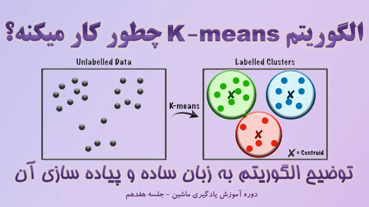
So first uh spectral clustering makes no assumption on the shapes of clusters. So you can cluster like any kind of a shape even intertwined spirals you will be able to find nice and neat clusters not to say other shapes however many other clustering algorithm like a c means or em tend to find non-convex shaped clusters then another advantage is usually em or like a k means source algorithm require an iterative process to find local minimum uh and they are very sensitive to initialization. So you usually need multiple restarts to get a high quality clusters.
However, spectral clustering where you have no such burden. Okay. Uh the general process of spectral clustering is partitioned into these three steps.
The first step is construct a similarity graph. For example, we can use Ken's neighbor based on their neighborhood using like a uklid distance or other distances you like to do your clustering. Okay. Then for all the points you can construct such similarity graph. For example, if you look at this illustrative example, you can see the original data points. If you do uh symmetric can neighbor you will find this k nearest neighbor neighbor graph like the following.
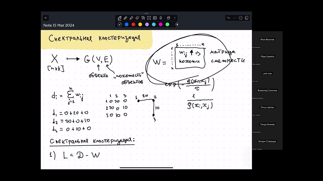
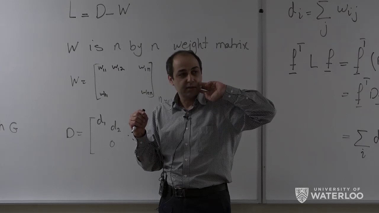
Then we can embed the data points in a low dimensional space using spectral clust embedding. What is this? This essentially is we can uh do graph llashing compute the igon vectors of such graph llashing. After this embedding the cluster structures become more obvious. Then we will be able to apply classical clustering algorithm like a game on these embedding. That means we will be able to partition the embedding graph into nice clusters. So this is the general idea. Now we look at how we do it step by step. First suppose we have a graph. This usually is obtained by the k nearest neighbor. Then we get a weights. Suppose the weight w sub one two is a weight connecting the vertices one and two. Okay. Then the adjacency matrix is n by n symmetric matrix like this one. Okay. Then the for each element what you got the the assignment is if there's a edge between like a one and two then you can based on the edge weight w sub one two you can get that weight w subig j is the weight of this cell okay if there's no connected edge like one and four is not connected then one and four this cell will be assigned as zero. Okay. Then we can perform llashing on this matrix.
Essentially is we use a diagonal matrix of degrees minus this adjacency matrix we'll get a laplash. Okay. What is diagonal matrix of the degrees? simply says you the degree is defined by for each row you just sum up all the degree all the weights or you say all the zero values uh in in this row for example for row one what you get is w uh sub12 plus w sub13 you get the weights that's the degree you will get okay that's d1 similarly for other degrees you is to calculate in the same way llian this matrix value is if this one is diagonal matrix I equals J then you get the D sub I okay that's the row uh value of this degree if the if it's other cells like I J has an edge then because zero minus this W subi J you get minus W subig that's what you get If originally was zero, you will still get zero. Okay. So that's the value you got from uh calculate this llashian matrix.
Then we can see how we can calculate the graphs for igon value and igon vector.
Okay. So we pro can see the igon uh value computation is based on these formula which has been used very popularly in linear algebra in matrix computation. Okay. We will not get into very detail but general philosophy is you get a matrix A. Lambda is igon value of A and for some vector V you follow this this equation and V is igon vector and the lambda is the igon value of A.
Okay. So then for a graph G if we have nodes then it's adjacency you will have n on values and this niggon value you can sort them according to the descending order you get lambda 1 lambda 2 to lambda subn uh of this n corresponding igon vectors will be x sub one to x subn.
uh you look at this figure one you probably can see this is the original graph you we have six uh vertices and their connections weighted connection is marked using those weight those values okay then obviously the the original uh matrix adjacency matrix is marked here you probably can see and that's the original adjacency matrix then we can calculate uh this originally a uh I this matrix on value and you probably can see this is their iggon vector and this is their igon value and you you you probably see this is mu one to mu6 okay so that's the spect spectrum of the graph okay then the value and igon vector of the graph. The graph llian of G is calculated you for this graph essentially is you get a lambda 1 lambda 2 to lambda n and we know the value lambda 1 lambda 2 lambda n we can sort them in this order. Okay. So if this zero uh you you get a spectrum is you you get this lambda value that's igon value and igon vector then value reveals a global graph property which is not apparent from the edge structure itself.
Essentially if you get a zero is the iggon value with k different igon vectors you probably will see these essentially is the k uh k com connected components that means if lambda y is zero that represent the one connected component. Okay. Then if a graph is connected then lambda 2 will be greater than zero. Lambda 2 is argebic connectivity of G. Here you probably can see uh RG air subg has lambda 1 lambda 2 lambda 3 as zero. You'll get a three connected components.
And if you have uh air this G1 and G2, you probably can see G1 uh is has only one connected component and G2 also has one connected component. That's why lambda 2 is greater than zero. However, you also can see G2 is much denser, much more connected than G1. That's why G2's lambda 2 value will be greater than G1's lambda 2 value.
Then we can work out the partitioning via spectrum methods. The general philosophy is if we got this original graph, we map them into laplashing of this original graph is this value.
Okay. Then we actually also know we can calculate the second the second igon vector and the second vector v sub 2 cor corresponding to lambda sub2 and for lambda sub 2 the smaller the better quality of the partitioning because if lambda is zero means it's not connected and if lambda 2 actually is greater means they they are more tightly connected. If you want to get nice partitioning, you want to find a smaller lambda 2.
Then if we calculate this uh uh for each node I in G, we can assign it uh the value then we v2 subi. So for for example these uh node one's v2 is 0.1 0.41 41 then if we want to find these are the six nodes their corresponding v2 value then if we get this uh v2's value uh we can get a greater than zero uh then we can assign to c1 and this v2's value is less than zero it could be another cluster then we actually will get a nice partitioning. Uh C1, C2, uh this 1 2 3 will become one cluster. Four, five, six will become another cluster.
So we can extend this algorithm to K partitions.
uh the in uh Jordan and uh and uh vice algorithm uh you know work out by Andrewing Michael Jordan and and this published in 2002 was a normalized uh llian essentially the original llian you see is not normalized but once you use this formula you can normalize the graph So the degree that part is all one and all the other rows you add up actually is minus one. So you finally get a normalized uh graph. So we can compute the first kig on vectors uh v1 to vk then we can calculate the the matrix the you you in a similar way we can do the partition into you know because we take the ice row of u as its feature factor after normalizing to norm one then we can cluster the points with k means into k clusters. Uh and this method is commonly used as a dimension uh reduction dimensionality reduction methods for uh clustering.
Up Next

Geometric Deep Learning: Graph Convolutional Networks Tutorial
@prof.alexbronstein6936
970 views•2020-01-20

Secure Multiparty Computation (MPC): Foundations & Challenges
@SimonsInstitute
7.3K views•2015-05-28

Bypassing Tor Censorship: Bridges and Pluggable Transport Guide
@Coding_ForEveryone
397 views•2024-06-11

Neural Networks Explained: Math, Layers, and Learning Fundamentals
@3blue1brown
21.9M views•2017-10-05
Related Study Plans & Knowledge Roadmaps
Structured learning paths in Artificial Intelligence