







![[딥러닝 기초] MLP Training1](https://i.ytimg.com/vi/064i6dKK_oQ/maxresdefault.jpg)
![(2024Ver) [인공지능 특강] 16강. 활성함수의 필요성과 오류역전파](https://i.ytimg.com/vi/US5Nu7iM_YY/maxresdefault.jpg)











![Neural networks [6.6] : Autoencoder - denoising autoencoder](https://i.ytimg.com/vi/t2NQ_c5BFOc/maxresdefault.jpg)












An autoencoder is a generative neural network model that learns to encode input data into a compressed low-dimensional representation and then decode it back to reconstruct the original input, commonly used for tasks like image compression; the implementation involves creating an encoder-decoder architecture where the encoder reduces data dimensions through successive layers (linear or convolutional) and the decoder reverses this process, with training optimized using mean squared error loss to minimize reconstruction differences between original and decoded images.
Implementing Autoencoders in PyTorch: Theory and Code
Added:Basic PyTorch mechanics, including creating Tensors, building custom models using 'torch.nn.Module', and writing standard training/optimization loops.
Foundations of Deep Learning, specifically feedforward neural networks (MLPs), activation functions, and backpropagation.
Core concepts of Convolutional Neural Networks (CNNs), including convolutional layers, pooling, and transposed convolutions (deconvolution) for upsampling.
An understanding of basic regression and classification loss functions, particularly Mean Squared Error (MSE) and Binary Cross-Entropy (BCE), which are used for reconstruction loss.
Variational Autoencoders (VAEs) to learn how to transition from standard autoencoders to probabilistic generative models.
Specialized autoencoder architectures such as Denoising Autoencoders (DAEs) and Sparse Autoencoders for robust feature learning and noise reduction.
Practical applications of autoencoders in industry, including anomaly detection, image inpainting, and dimensionality reduction for complex datasets.
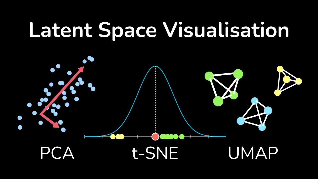
Latent space exploration, visualization, and manipulation techniques using methods like t-SNE or UMAP to evaluate the learned bottleneck representations.
Generative Adversarial Networks (GANs) to explore alternative and highly competitive generative modeling paradigms.
85.8K views2.4Klikes30:00Original Release: 2021-03-22
welcome everyone today we're going to learn about auto encoders and how we can implement them in pytorch auto encoders are really cool and the mechanism is actually pretty simple in this case we deal with an input image and we want to encode it to get a low dimensional embedding of the image and after that we want to decode it again and reconstruct the original image as good as possible so that's the whole mechanism behind it so we deal with the original image get an encoded image and reconstruct the original image again a very cool possible application for this is for example video compression where we want to send over the images over the network from one end to the other end so instead of sending the whole image we could simply send the encoded data only and on the other side we then have the decoder stored and can decode the image again this would save a lot of cost and could be much faster and i think this is pretty cool so how do we encode and decode the image for both operations we can simply use a feed forward neural net or when we deal with images we often use a convolutional neural net which usually performs better and later i will show you how to code both versions in pytorch when we speak about such a model we call this a generative model because here instead of doing a classification at the end we want to generate images based on the encoding so in order to train our model we need a loss function that we want to optimize we want our reconstructed image as close as possible to the original one so all pixel values should be almost the same so our loss function is simply the mean squared error which calculates the difference between all intensity values sums over all pixels and then calculates the mean value now here's a little trick in order to understand the whole process better instead of thinking about all transformations as operations in one way we can think of this as a circular or fourth and back operation we encode in one direction and then we want to go in the opposite direction and decode it again to get the original image so for each transformation we apply in the encoder we want to apply the inverse of this operation in the decoder for example if we apply a linear layer that reduces the size the reverse operation is also a linear layer that increases the size again now for cnns this is a little bit trickier here we apply convolutional layers so the inverse is actually called a transpose convolution pi charge has this layer already included for us so we can simply use the nn.conf transpose 2d layer the only tricky thing with this is to determine the correct input and output shapes but i will show you how to do this later alright so that's everything we need to understand auto encoders now we can jump to the code and if you enjoy this content then i would be very happy if you hit the like button and subscribe to the channel all right so here we are in a two-parter notebook and we already have all the imports that we need so we have torch we have torch nn torch optim we have data sets and transforms from the torch vision module and we have matplotlib to plot the data later and then the first thing we want to do is load the mnist data and for this we use a data loader and if you don't know how a data loader works then i will link a tutorial where i explain this here so we define a data loader and we can give it a batch size here and we also define the data set so this is included in pi touch and we get this by saying data datasets.mnist and this will download the data and store it here in the data folder and we also can apply a transform here and in this case we simply apply a to tensor transform so this will transform the images to a pie touch tensor and i pulled this out here because this is actually important for our model later so later i also want to show you uh what we have to consider when we use a different transform here so we will get to this later but for now what we want to keep in mind is how our data looks like so what values do our mnist images have so let's actually run this and let's inspect the first images or the first batch so we get the first batch by creating a iterator object like so we say data iter and then we call iter with our data loader and then we pull out the first images and labels by calling data dot next and then we want to print the minimum and the maximum value and we get this with torch.min of our images and also torch dot max of our images so let's run this and then we see the values range from zero to one so this will be important for our model later and this might change if we also change the transforms here so we will learn how to do this later so with this in mind that the values are between 0 and 1 we can create our auto encoder class so let's create a class and let's call this auto encoder and this is our model so we have to inherit from nn.module and if you don't know how to do this then i will link another tutorial here where i explain how you create your pytorch classes so the first thing we want to implement is the init function and this only gets self and then we also want to implement the forward pass and this gets self and x so for now we only say pass and in the first example i want to show you a simple feed forward neural net with linear layers and a few hidden layers and here what we want to do is we want to repeatedly reduce the size so in the beginning our images have the size n and then by 785 so this is 28 by 28 because and this is how many it pixels the images have in this data set and n is our batch size so now we want to reduce this with a few linear layers and a good way to structure your code in an auto encoder is to use a sequential model so first we create a n coder and this is a n n dot sequential model and now here we want to repeatedly apply linear layers so let's create a first linear layers and the input size is 28 by 28 so this is 784 and the output size here we can play around with different sizes so as first output size i want to use 128 so what this is doing is this will reduce the size from [Music] n by 784 will reduce it to n by 128 after this we also want to apply a activation function so here we use nn.relu the most popular one and let's move the comment up here again and now we want to do this multiple times so now we want to create another linear layer and this time our input is 128 and as output we can choose a different smaller size so here i use 64 and then again we want to apply the relu activation and then let's do this a couple more times so let's actually um copy and paste this so we create another linear layer and here we use 64 and as output let's use 12 then again we have the relu and now we create one last linear layer so nn.linear and here we use 12 and as output size let's use three and then as the last layer here we don't need an activation function so let's remove this again so now this is our sequential model for the encoder and the final output size here is n by three so this will drastically reduce the size of our input images from this size to only this size and then later we are able to almost perfectly reconstruct this again so this is really great so yeah this is our encoder and now we want to do the same thing in the opposite direction so let's copy this actually and say this is our self dot decoder so here we want to go in the opposite direction so here we want to go from n by 3 all the way again until n by 784 so let's remove the comment here and so now we basically we want to look at all the linear layers and switch the sizes so here the input size is 3 and the output size is 12. then here we have 12 and 64. here we have 64 and then as output size 128 and here we have 128 and as output size 28 times 28 and now we also here we apply relu actuation functions in between and now for the last layer this is actually important so here we have to apply another actuation function so let's go back to our data set and have a look at this so we know that our images have values between zero and one so we now we need an activation function that puts the values in exactly this range so in this case the one million dollar question is which actuation function do we need to get outputs between zero and one so this is the sigmoid function so we get this by saying n n dot sigmoid so this is what we need as last layer so keep this in mind so now we have our encoder and our decoder and in the forward pass we simply apply both of them so we say encoded equal self dot in coder and this gets x and then we get the decoded again by calling self.decoder and this gets the encoded as input and then we simply return the decoded image again and yeah this is all we need for our encoder class so as a note here note keep the last layer in mind for example let's say our our input images are in the range minus one and plus one then we don't need the seed point here so in this case we for example want to apply the ton h function and this might actually very easily happen if you apply a normalization here so let me quickly show you how to do this and that's why i pulled this out so let's say our transform is transforms dot and then compose and here we can give it a list so the first one is again the tensor transform and then we also apply transforms dot normalize and here we want to use 0.5 for the first dimension and for the other dimension we want to use 0.5 as well so now if we comment this out so let's actually run this and then also run this again and have a look at torch min and max then we see we get the range from minus one to plus one so that's why we always want to analyze our data first and want to know what are the ranges and then here we might use for example the ton h so keep this in mind so now i will comment this out again and we simply use the trans to tensor transform and now we have our images in the range 0 and 1 again so now here we created our encoder so now we actually want to set this up so we create a model and say this is our encoder then we also need a cry criteria and i already told you that this is simply the mean squared error loss so we get this by saying nn dot mse loss and we also need a optimizer so optimizer equals torch dot optim and here let's use the atom optimizer and we want to optimize the parameters of our model and we also need a learning rate so here let's use one e minus three so point zero zero one and also if you want to you can give this a weight decay so weight underscore decay equals and let's use one e minus five so you can play around with these numbers and see which performs better so let's run this cell and now we get an error and this is because in our init function of course we have to call super dot underscore init and initialize the um super class so i always forget this when i record tutorials so let's run this again and let's run this again and now this works and now we do the training so for this i simply copy paste this here so if you don't know how the training loop works then i will link another tutorial here where i explain this so basically we define the number of epochs and then here i will set this to 10 because this might take a few minutes to train if you don't have a gpu so you can of course increase the size if you want to have more accurate um values then we create a list to store the outputs then we iterate over the epochs and then we also iterate over our data loader and now here we want to reshape the images in our first example because the images are in the shape 28 comma 28 and we want to have this in size 784 so that's why we apply this then we call the model and get the reconstructed image then we call the criterion with the reconstructed image and the original image and calculate the mean squared error and then we have to be careful to always zero our gradients and then call lost backward and an optimizer step and then we also want to print the epoch and the loss after each epoch and we want to store the epoch the image and the reconstructed image in the outputs list so let's run this all right so training is done and our loss slowly decreased so it's still not that low but maybe you might want to increase the number of epochs but it's working and let's actually have a look at how the reconstructed images look like so let me copy and paste a simple function here that will plot the images so we will plot the images every fourth epoch and create a figure and then we get the images and the reconstructed images from the outputs array that we stored and this is a torch tensor so we want to call detach and then convert it to a numpy array here for plotting and then we iterate over the images and plot the first nine images and here we want to be careful so here again we want to apply the reshaping again in the reverse direction so here we went from 700 from 28 comma 28 to 28 times 28 and here we want to go in the do the opposite so we do 28 comma 28 and then we simply plot this so here our data has to be in this format so let's run this and we see so this is after the first epoch and we can almost assume the correct number but it's very blurred and then it's getting better after the next four epochs and i think this is after um eight epochs so then we see this um image and we see that the result is still a little bit blurred but it's actually pretty good so we can detect which number this is and i think this is pretty good for a simple linear layer that um reduces to the size to only three output layers so i think this is pretty cool yeah so this is the first example i want to show you and now we want to use a convolutional neural network and see if we can improve the performance even more with this so let's run this again and create a new cell and then let's actually copy and paste this class and put it down here and for the first auto encoder let's rename this to auto encoder underscore linear and this will be our cnn auto encoder so here we do the same thing and now the first we want to do is now here we actually put them in as 28 by 28 so in our training function training loop we can remove this reshaping and also later for plotting we can remove this as well so let's do this first and yeah so now we can continue here so now instead of linear layers what we want to have here is convolutional 2d layers so here we can say nn.conf and then 2 d and here we have to give it input channel and output channel so this is one and then you can play around with this size so let's use 16 as the first number of output channels and then we also have to give it a kernel size so here we use three then we can give it a stride so this is two and let's use a padding equals one so this is our first convolutional layer and then as well here we want to apply reload activation functions then let's create another convolution then again the relu and then let's use another convolution and actually let's get rid of those here so we only want to do three passes and now let's simplify this a little bit and get rid of this so now it gets a little bit tricky because now you have to be careful to get the correct shapes and the correct input and output channels so again if you don't know how these convolutions work then i will link the tutorial about the cnns where i explain this so actually let's inspect the input and output size so the input for this is n by 1 by 28 by 28 so this is why our first input size is 1 and then after that we get 16 and for the size we get 14 by 14 so we reduce the size of our images by 50 and then for our next one as the input size we have to get the output channel size of the previous one so this is 16 and then here we can actually increase this and use twin 32 and we will keep the rest and then again let's have a look how this will look like so this will be n by 32 by seven by seven so again we reduce this in half and then again we use a relu and then again a convolutional and this will have 16 uh let's actually increase this again so 64. so here we have 64 output channels and then um here we want to use let's use seven so we have one by one as the output size of our image so basically only one pixel but 64 channels so we increased the channels but we reduced the size of the image so now this has far more parameters than this size so this is our encoded version and now we want to go in the backwards direction with the conf transpose 2d layers that i mentioned so here let's copy and paste this to know with what size we are working here so now um we apply the n n dot conf transpose to d and now here we again have to switch the um sizes and here i made a mistake through copy and paste so here this input size must be the output size of this one so here we have to say 32 and then 64 and seven and here we do the opposite so we have 64 input channels and 32 outputs channels and the kernel size is seven so this will give us the size n by 32 by seven by seven so like we have here so this is correct then again we use a relu and now let's use another conf 2d conv transpose 2d and here we switch this convolutional layer so here we have 32 as the input and 16 as the output and a kernel size of three and now if you run this then this will actually give you a size of n by 16 by 13 by 13 and what we want we have 16 by 14 by 14 so we need plus one so this is a little bit tricky so i recommend to play around with these ones and have a look at what they generate and now in order to compensate this we can give it a parameter and here let's actually let's say let's use the exact same stride and padding that we have here stride equals two and padding equals one and then we can say output padding equals one so this will put um zeros in it so that you get 14 by 40 now so yeah this is a very important thing to know to use the output padding parameter and now again we use the relu function and then we use another conf transpose to d and here we have to revert this one so as the input we use 16 and as the output we use one and then again we have the same kernel size the same stride and the same padding and now here will happen the same thing so if we don't use this then we get n by 1 by 27 by 27 so then again we need the output padding and then we get n by 1 by 28 by 28 and then we don't need these anymore and again as the last layer we want to have the sigmoid so the same as before and now this is no longer correct so yeah this is how we implement a auto encoder with convolutions so we need the convolutions and then in our decoder we use conf transpose 2d and be aware that you use the correct shapes and also maybe use an output padding if necessary so let's run this and here i actually want to mention one more thing so a lot of times in convolutional neural networks you use the max pool 2d function so nn.max pool 2d this will essentially reduce the size and to revert this there is also a function that is called nn nn.max un pool 2d so this is what you might want to use in the decoder then but you don't need to do this um you can also for example play around with different strides and paddings and kernel sizes the only thing you want to make sure is that at the very end you get the same output shape as you had in the beginning so yeah keep that in mind and now let's run this and now let's create our new model with the convolutional auto encoder so let's run this again and then again let's run the training and see how this performs all right so our training is done and again our loss decreased and now this time it's much better than before so i guess before we had point zero three something and here we have point zero zero something so this is much better so yeah we can see that our c and n's usually perform much better than a simple feed forward neural net with linear layers so let's actually run our plotting loop again and let's plot some example reconstructions so we can see that after the first epoch it's a little bit blurred but it's already very good and then this is after the fourth and after the eighth epoch and we can see that already here the reconstruction is pretty good so yeah i think it's almost the same image so yeah this is really cool and this worked so yeah this is how you implement a auto encoder with pytorch and i really hope that you enjoyed this tutorial and if you want to have a small exercise then i can give you the exercise to apply the max pool 2d max pool 2d and the unpooling that i mentioned and you can also try to inspect the encoded data and see if this can actually be plotted and how this looks like so yeah this is something you can try out for yourself and then i hope to see you in the next video bye you
Up Next
24:19
PyTorch LSTM Autoencoder for Time Series Anomaly Detection
@onepagecode
522 views•2024-09-03

57:48
Secure Multiparty Computation (MPC): Foundations & Challenges
@SimonsInstitute
7.3K views•2015-05-28

13:03
Bypassing Tor Censorship: Bridges and Pluggable Transport Guide
@Coding_ForEveryone
397 views•2024-06-11

18:41
Neural Networks Explained: Math, Layers, and Learning Fundamentals
@3blue1brown
21.9M views•2017-10-05
Related Study Plans & Knowledge Roadmaps
Structured learning paths in Artificial Intelligence
artificial-intelligence
Aligning LLMs: DPO, TRL & Custom Datasets
01Foundations of Python & Machine Learning
02Transformers and Large Language Models (LLMs)
03Aligning LLMs: SFT and RLHF
+ 3 more learning modules
24h6 modules
Explore Roadmap
artificial-intelligence
Federated Learning: PyTorch, Flower & Privacy
01Python & Machine Learning Foundations
02Deep Learning Basics with PyTorch
03Introduction to Federated Learning
+ 2 more learning modules
35h5 modules
Explore Roadmap
artificial-intelligence
Securing LLMs: Guardrails AI & NeMo Gateway
01Introduction to LLMs, Python, and APIs
02Understanding LLM Vulnerabilities & Threats
03Defending LLMs with Guardrails AI
+ 2 more learning modules
15h5 modules
Explore Roadmap
artificial-intelligence
Building Recommenders: Two-Tower & Vector DBs
01Foundations of Python & Machine Learning Basics
02Introduction to Recommender Systems
03Deep Learning & Representation Learning
+ 3 more learning modules
75h6 modules
Explore Roadmap