
























Likelihood is a statistical concept that measures how well a given set of parameters explains observed data, and it is proportional to probability but not identical to it; unlike probability which predicts data from known distributions, likelihood evaluates how well different parameter values fit the data, and Maximum Likelihood Estimation (MLE) finds the parameter values that maximize this likelihood function, serving as a fundamental technique in statistical modeling and machine learning for estimating model parameters.
Likelihood vs Probability: The Math You Should Know (MLE)
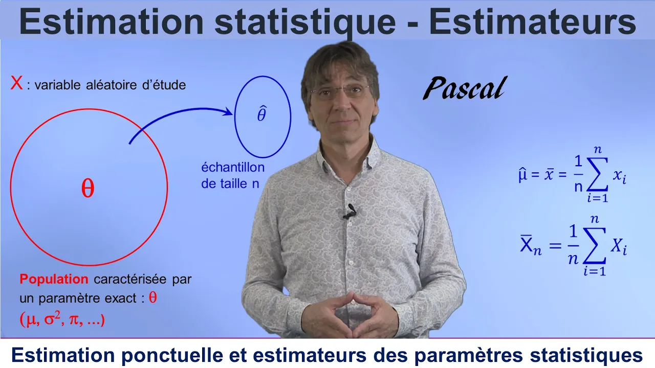
Added:Basic Probability Concepts: Familiarity with probability density functions (PDFs), probability mass functions (PMFs), and joint probabilities.
Fundamentals of Calculus: Understanding derivatives and basic optimization techniques, specifically how to find the maximum of a function by setting its derivative to zero.
Common Probability Distributions: Knowledge of standard distributions such as the Normal (Gaussian), Binomial, and Bernoulli distributions, including their key parameters.
Properties of Logarithms: Understanding logarithmic rules (e.g., converting products to sums) to comprehend why log-likelihood is used during optimization.
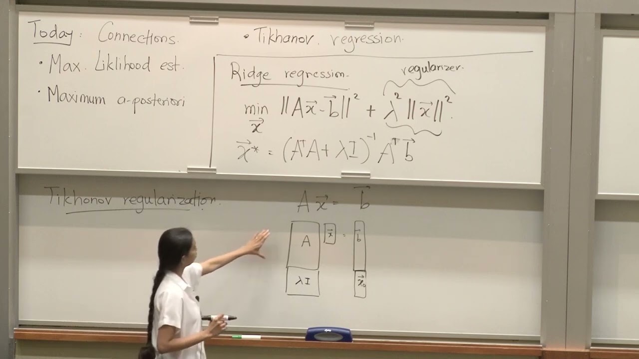
Maximum A Posteriori (MAP) Estimation: Exploring the Bayesian alternative to MLE, which incorporates prior probability distributions into parameter estimation.
Loss Function Derivations in Machine Learning: Learning how MLE is used to formally derive standard machine learning loss functions, such as Mean Squared Error (MSE) and Binary Cross-Entropy.
Estimator Properties: Evaluating the quality of estimators by studying concepts like bias, variance, consistency, efficiency, and the Cramér-Rao Lower Bound.
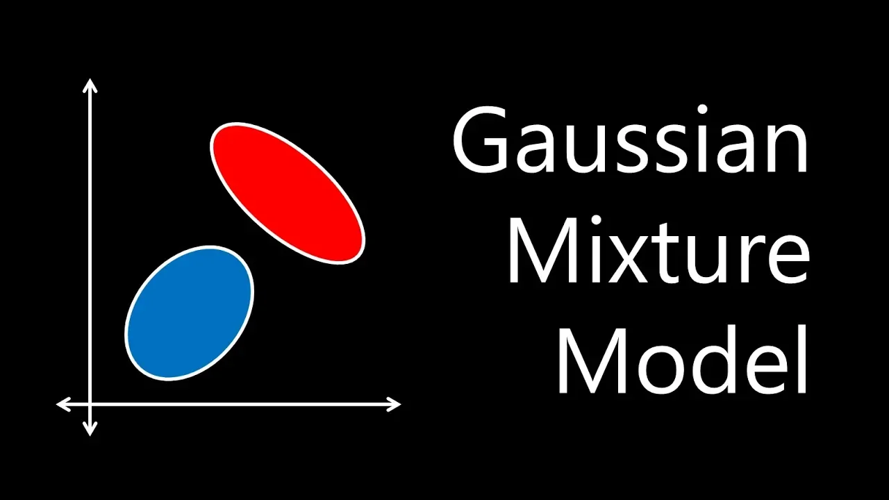
The Expectation-Maximization (EM) Algorithm: Applying MLE principles to complex latent variable models, such as Gaussian Mixture Models (GMMs).
72.7K views2.4Klikes27:48Original Release: 2022-07-28
hello everyone and welcome to a special episode of code emporium where we're going to talk about likelihood so likelihood is one of those terms where it is proportional to a probability but it is not quite a probability and it's pretty confusing so we're going to walk through some intuition walk through a formal definition and then also we're gonna work through a lot of math and so i have my trusty pen here so let's get to it all right so let's actually start this discussion by explaining the difference between probability and likelihood so right now i'm going to draw a 2d graph we have the y-axis and the x-axis over here and this x-axis i'm gonna say is going to represent prices of houses so let's say that this could be two hundred thousand dollars then we have four hundred thousand dollars then we have six hundred thousand dollars and this x-axis just goes on and then the y-axis is going to represent a probability which i'm going to represent as p of x and let's say that you know for some given population we just know that the distribution of all house prices will look something like this blue curve where you have a lot of examples that probably have middle to to lower prices but then there's like a few examples when you get to the tail end that'll be like really expensive houses and for all intents and purposes let's say that this is going to be some log normal distribution or something very close to it which means that well we can represent this here with a mean and a standard deviation which we'll call mu and sigma now because this is a probability distribution we know that it can exhibit certain properties like one such property is that the total area under this blue curve is going to be one so in fancy mathematical notation we could write that as the integration over all x and it's going to be the probability p of x d x now this entire integration for over all values of x is going to be one and something else that we can also define with probability is well the range of values so for example let's say that i'm going to draw a line at 400k and i'm also going to draw another line at around 300k and we have this shaded region over here now one statement we can make now with probability is let's say that the area under this region in this yellow region is 0.35 so we can say the integration where the values of x lie between three hundred thousand and four hundred thousand the probability values if you sum them up dx this is going to be 0.35 and so with the notion of probability we can make statements like this where it's basically saying given some distribution or rather given like the mu and the sigma of some distribution the probability that a house price is between 300 000 and 400 000 is 0.35 so that's kind of the notion of probability but let me try to now relate this to likelihood by drawing the same exact graph all right so now i drew an x-axis of prices and a y-axis of probability values and in this case maybe the probability values are going to be of the order 10 to the negative 7.
so likelihood likelihood is essentially not a probability but it is proportional to a probability and what i mean and why it is actually useful is because in many situations we're not given this blue curve like we don't know what the value of mu and sigma is but instead we are given data points where we might have like some houses let's say one house is like ninety thousand dollars then we have a few houses in like the two hundred thousand dollar range and maybe a few a little above five thousand and then like some stray one close to a million way out here now in this situation let's just say at this point we randomly want to find some distribution that fits this data and in this case we'll randomly assign the mu here and the sigma here to be some value so i'm going to say like let's just say the mu i'm going to change this color to uh a blue line so this mu let's just say that it's going to be 14 and the sigma is going to be 0.4 just for an argument's sake now in this situation we might get a curve that looks something like this dotted line now how well does this curve with a mu of 14 in a sigma of 0.44 how well does this curve fit this data that is quantified by likelihood and so we can write the likelihood function we're going to call it l the likelihood function is going to take as parameters the parameters of like the distribution itself and it's going to say okay the likelihood of like mu is equal to 14 and sigma is equal to 0.4 for this given data let's say that it is 3.72 just for an argument's sake now we can also just play around with these mu and sigma values they're parameters to some function anyways so let's just say for another argument's sake i'm going to call it mu let's change it to like 15 and sigma we'll just i don't know we'll keep it at 0.3 or something like that and in this case we might get a curve that looks something like this and it's here that we can say maybe the likelihood that the mu is 15 and sigma 0.3 how well this green curve essentially fits this blue data will be quantified by this function and let's say that it's going to be 2.8 and similarly we can have another function we'll represent it with yellow that looks something like this and this could be like a mu is equal to 15.5 and then we have a sigma equal to 0.4 and we can say here the likelihood function that's the likelihood like how well does this new distribution now fit the given data this could be some i don't know 2.6 and what now this can tell us is well this this number here that is the 3.72 is the greatest of all of the three distributions for this data which means that this blue distribution over here fits these data points the best and you can kind of see here that in machine learning we are given this exact same scenario where we are given data points like this and we kind of want to find some distribution that fits the given data the best and so i hope this is a little clear if like how likelihood is going to be different from a probability with probability we are given a distribution and we can make statements about the data with likelihood we are given the data and we can make statements well about how well the distribution fits the data by passing in these parameters and so now let's talk about likelihood but with a much more formal definition alrighty so this definition of likelihood i took from a book that was written by a famous mathematician or statistician ronald fisher and in it he defines likelihood very precisely as the likelihood that any parameter or a set of parameters should have any assigned value or set of values is proportional to the probability that if this were so the totality of observations should be that observed let's break this down and convert it into some mathematical notation now so the likelihood right here the likelihood that any parameter these are these are keywords should have any assigned value so let's let's start with that so right now i'm going to change my color to this is the likelihood function and any parameter or set of parameters is going to be the parameters of the distribution that we can set right so i'm going to toggle this with a green color we'll call this mu and sigma in this case so the likelihood that any parameter should have any assigned value so if we assigned this to a value let's say if we assigned this to be equal to like i don't know 14 and assigned this sigma to be equal to 0.3 then this value is going to be proportional to the probability that if this were so so let's just break it down there it's going to be proportional to the probability that if this were true if the mu and the sigma were if the mu was 14 and the sigma of the log normal distribution were 0.3 then the totality of the observations here would be that observed so the totality of the observations would be all of the data points that were given typically in i don't know in machine learning it's going to be like all of our training data but even in the previous example it's going to be the set of house prices so that is going to be like y 1 y 2 y 3 and let's just say that there's i don't know some 10 000 examples and each of these would have assumed some value right because this y1 could have been i don't know some house price that's 238 thousand dollars and this y2 over here could have been some house price which was four hundred thousand dollars and like so because all of these values would have assumed some house price and this is all going to be the joint probability distribution that all of this is true and typically we would also parameterize it well all of this is given that we are observing mu and sigma so that if this were true i think it says here that if this were true the totality of observation should be that observed so if this were true which means let's make this true that is given the value of well mu and sigma and these specifically are going to take on the values that we would have passed over on this side so it's going to be 14 and 0.3 so that means that the likelihood that well let's say that we pass in a parameter of the distribution to be 14 and 0.3 this likelihood value is going to be proportional to the probability of observing all of these examples such that well we are assuming the actual distribution that is we are assuming the values that we passed are mu with 14 and sigma of 0.3 and so i hope that this definition now is becoming a little more clear and we're able to break this down into mathematics because from here on out we're going to be using this in well the world of machine learning so i hope this is clear let's now consider a machine learning problem where we want to predict the value of a house price given some information about the house and this information could be information like square footage or it could be number of bedrooms the age of a house and so many other factors and all of this information we want to model it model it with let's say i don't know a linear regression model but it can be essentially any kind of model that has parameters any parametric model now in this situation we would describe this model mathematically as y which is the house price this is going to be equal to i'm going to call the parameters of this linear regression theta because that's quite standard notation theta 2 times i'm gonna start with the number of bedrooms so i'll call it hashtag bedrooms and we're going to add to this let's say theta 1 times and we're going to call this other term and let's say that we pass in the age of the house as well and for now let's just say that these are the only two parameters that we passed but there could be plenty more and we want to add to this a constant term so i'm going to call it theta zero and then we also have some epsilon which is going to be an irreducible error probably because of inherent model noise or also because bedrooms and age are probably just not enough in order to predict um the accurately like what a house price could be now this here this entire equation is typically called the hypothesis all right now to this linear regression hypothesis let's actually see where the concept of likelihood really comes into the picture so let's look at this function which is l and we know that the likelihood function is going to be a function of parameters so that's theta 0 theta 1 and theta two now what this function over here is going to decide is it's going to quantify that if we were to set the value of theta zero theta 1 and theta 2 to some specific value it's going to give us a number and that number will quantify how well this assumed distribution is going to fit that data but when we're doing like machine learning and remodeling we don't want to just find a number we want to find the best number we want to find the best fit of data in other words we want to maximize this likelihood function and we're in essence not really concerned about the value of likelihood itself but we are concerned with what are the values of theta that are going to maximize this function and in mathematics we determine that with arg max we represent it with arg max and what we want to do is we want to determine the values of theta 0 theta 1 and theta 2 that will in essence maximize the likelihood function i'm going to now represent this with hats all these thetas with hats because in the end they are estimations and i'm also going to call it m l e to stand for maximum likelihood estimations because in essence these are the values of the theta terms that maximize the likelihood function i'm also going to add just for the save completion of notation theta 0 theta 1 and theta 2 under the arg max just to show that we are maximizing across the theta terms and any other term that comes in this likelihood function whether it's a set of x's that is the house information or the set of prices which is the y's all of them should not they should remain constant with respect to this maximization now this term here looks very cumbersome and so we would typically minimize that or optimize this using well typically vectors so let's just say let the theta vector we're going to call it theta equal to theta 0 theta 1 and theta 2.
and writing rewriting now this equation we can now rewrite it as let's call it theta is equal to arg max of the theta term and we're going to write the likelihood function and for the sake of completion we're going to put a hat and mle to signify it is an estimation and it is now this function that is going to be the basis of all calculations that we will make in this video and also typically of parametric models and how you would want to solve for parameters in a model with well maximum likelihood estimation which is exactly what this technique is it's very clear now that the likelihood function is useful in mathematics so let's actually further break this down using the probability notation that we introduced when defining likelihood so we know that the likelihood of let's say now we can say theta because we know that the parameters are represented by theta this is going to be proportional to the probability of let's say our training data is a set of house prices so i'm going to represent that with y 1 which is some value and then y 2 and so on until y 10 000 because we had 10 000 training examples and in standard notation we are given the values of theta so this is standard notation these values can take on some house prices and this is some assumed value that we would we would just like plop in but we can assume house prices are independent of each other and in math notation we call this iid that is independently and identically distributed which means that a house price does not depend on another house's price in our 10 000 example data set which is a very standard assumption to make and because of this we can now write this probability which is a joint probability distribution in terms of individual product of probability distributions and so i represent the individual probabilities with a small p over here and now we can represent this in a more concise notation with the product symbol where we range i is equal to 1 to 10 000 and then take a product of all of these product terms now this is a good notation right now but computationally speaking this can lead to something called arithmetic underflow and why this is the case is let's assume that you know this price over here is going to be a probability so it's going to be some number between 0 and 1. let's say that it is i don't know for the sake of the argument 0.83 this one over here is going to be something like 0.74 this one over here is going to be 0.56 and when you're taking the product of multiple numbers that are under one you are going to get a value that is going to be extremely close to zero so close to zero that computers these days just won't have the precision to deal with those numbers and so this term is not easily manageable and in order to deal with the situation we would like to convert it into some summation form and we can do that by taking the logarithms on both sides and so you'll get a term that looks like this where i've just taken the logarithm and put it in brackets now if you expand the logarithm here you're going to get a log of products but we know that that's going to be the same as the sum of logs and so now we write the summation symbol across all values of i and it's at this point that we take the logarithm into our brackets here and we're going to put a big bracket and it's going to be the log or sum of logs of the individual probabilities here now this is a a very important equation here because what we really care about remember in the beginning was the original values of theta that maximize this likelihood function so we really just cared about this equation and we know that this is basically we need to maximize the likelihood function now something that we can kind of look here is that the value of likelihood over here is proportional to this term here and so they have the same maximum in fact something i didn't mention before was that we're able to take logarithms on both sides for proportionality because they logarithms are monotonically increasing which means that for a given a greater than b then this implies that the log a should be greater than log b and this is the property of monotonically increasing functions and so right now the value of theta that maximizes the likelihood is going to be the value of theta that maximizes this log likelihood which because it's not proportional to this term it's going to be the value of theta that maximizes the sum of log probability values and so if we were to simplify this term we would get the value of theta that gives us the maximum likelihood estimation and this can be used in our parametric model now from here like how do we actually simplify this well i'm not going to work out all of that in this video and that can probably be for future videos but essentially it all hinges on this clearly this probability distribution value right and for linear regression we would make the assumption that this is normally distributed and because of that we have like the probability density function for a normal distribution that we would write out and simplify and it's actually fun because if you do that as an exercise you'll see that it becomes the residual sum of squares and similarly if you do this for logistic regression you could use this would now probability function would now turn into the sigmoid function and the link function and you'll use concepts such as like if it were a binary classification you know that if the probability of it being in one class is the probability of is the inverse probability of it being in another class so that's one minus probability of the other class and you would use those kind of statistical tools and statistical rules in order to simplify this function and eventually get the value of theta but for all intents and purposes this is a lot better starting point because now it no longer suffers from arithmetic underflow and i hope now it is clear how maximum likelihood estimation and in just general the concept of likelihood is very useful in statistical modeling and i hope you enjoyed this video there's going to be a blog post that accompanies this video too so if it's not there as soon as it's uploaded it'll be there eventually very soon thank you all for listening and i hope you enjoyed this video bye
Up Next

48:49
Bayesian Statistical Inference I | MIT 6.041 Probability
@mitocw
187.4K views•2012-11-09

4:43
Elliptic Curve Cryptography Explained: ECC, ECDSA, ECDH
@PracticalNetworking
28.5K views•2024-10-21

10:44
Fourier Series Introduction: The Big Idea Explained
@DrTrefor
387K views•2021-05-03

6:00
The Mathematical Impossibility of Accurate World Maps
@Vox
23.3M views•2016-12-02
Related Study Plans & Knowledge Roadmaps
Structured learning paths in Mathematics
mathematics
Tensor Calculus: Vectors to Riemann Curvature
01Mathematical Foundations: Linear Algebra & Calculus
02Covectors, Dual Spaces, and Tensor Basics
03The Metric Tensor and Index Gymnastics
+ 2 more learning modules
40h5 modules
Explore Roadmap
mathematics
Gödel's Incompleteness: Logic, Proofs & Limits
01Introduction to Formal Systems & Hilbert's Dream
02Set Theory, Cardinality, and Cantor's Diagonal Argument
03Arithmetization and Gödel Numbering
+ 2 more learning modules
14h5 modules
Explore Roadmap
mathematics
Galois Theory: Fields, Groups & Solvability
01Foundations of Abstract Algebra: Groups & Fields
02Polynomials & Field Extensions
03Splitting Fields & Symmetries
+ 2 more learning modules
24h5 modules
Explore Roadmap
mathematics
Non-Euclidean Geometry: Models & Geodesics
01Euclid's Fifth Postulate and the Birth of New Geometries
02Hyperbolic Space and the Poincaré Disk Model
03Geodesics: Defining Straight Lines in Curved Spaces
+ 2 more learning modules
15h5 modules
Explore Roadmap