Einstein derived the quantitative theory of Brownian motion by analyzing the excess molecules crossing a cylindrical surface in a medium with concentration gradient, showing that the net flux equals the negative of the concentration gradient multiplied by the diffusion coefficient (J = -D(dn/dx)), where D is the diffusion coefficient.
Einstein's Theory of Brownian Motion | Derivation & Notes
Added:Deep Dive
Fundamentals of the kinetic theory of gases, including thermal energy (kT) and molecular collisions.
Kinetic Theory of Gases//Basic Assumption (or Postulates)//Molecular Collisions//Thermal Physics
566
The Kinetic Theory of Gases is based on ten fundamental postulates: (1) Gases consist of tiny spherical molecules that are identical within a gas but different between gases; (2) The distance between molecules is much larger than their size, allowing them to be treated as point masses; (3) Molecules undergo constant random motion with velocities ranging from zero to infinity; (4) All collisions between molecules and container walls are perfectly elastic, conserving total kinetic energy; (5) The mean free path is the average distance a molecule travels between successive collisions; (6) Collisions are instantaneous events with negligible duration; (7) Molecules do not exert attractive or repulsive forces on each other, meaning potential energy between molecules is zero; (8) The number of molecules per unit volume (number density) is constant everywhere within the container.
Click to watch →

Class 11 Full Term 2 Physics in One Shot | Unacademy Class 11 & 12 | Anurag Tyagi
123.2K
Kinetic theory explains molecular collisions: the collision frequency depends on molecular speed and number density. The collision cross-section depends on molecular size. This explains gas viscosity and thermal conductivity.
Click to watch →

HEAT 6 MARKs in ONE SHOT🔥| Complete Formula , Tricks , Questions
50K
Kinetic theory assumes molecules are small, elastic, spherical, identical in mass and size, moving in random directions with perfectly elastic collisions. Pressure results from molecular collisions with container walls. Root mean square velocity v_rms = √(3PV/M). Average kinetic energy per molecule is (3/2)kT; total kinetic energy is (3/2)nRT. Degrees of freedom: monatomic (3), diatomic (5), linear triatomic (7), non-linear triatomic (6). Ideal gas equation PV = nRT. Specific gas constant R_specific = R/M. Boltzmann's constant k = R/N_A = 1.38 × 10^-23 J/K. Law of mixing: T_final = (n₁T₁ + n₂T₂)/(n₁ + n₂).
Click to watch →

Kinetic theory of gases and radiations | 2025 MHT-CET PYQs
501
Kinetic theory assumes elastic collisions between gas molecules where both kinetic energy and momentum are conserved. This explains why gases maintain temperature during collisions. The number of molecules in a gas sample is proportional to PV/T, so reducing volume by 5% requires increasing pressure by approximately 5.26%. For two blackbodies radiating equal power, their radii and temperatures must satisfy r₁T₁² = r₂T₂². These principles form the foundation for understanding gas behavior at molecular levels.
Click to watch →

TÓM TẮTTOÀN BỘ VẬT LÍ 12 ( CTM) ÔN THI TỐT NGHIỆP NĂM HỌC 2025
77.4K
Gases consist of molecules in constant random motion with intermolecular forces. Key assumptions: (1) molecular size is negligible compared to intermolecular distances, (2) molecules move randomly, (3) collisions are elastic (conserving momentum and kinetic energy), (4) average molecular speed is v_rms = √(3kT/m). Pressure arises from molecular collisions with container walls. The ideal gas equation PV = nRT describes gas behavior, where n is moles and R is gas constant (8.31 J/(mol·K)). For 1 mole at STP, volume is 22.4 L.
Click to watch →
Deep Dive
Fick's laws of diffusion, which describe how concentration gradients drive macroscopic particle flux.

Fick's First Law of Diffusion
280.3K
Fick's First Law of Diffusion describes how particles move from areas of high concentration to low concentration, stating that the flux (J) of particles across a surface is proportional to the negative of the concentration gradient (ΔC/ΔZ), with the proportionality constant being the diffusion coefficient (D_AB): J = -D_AB × (ΔC/ΔZ). The negative sign ensures that flux is positive when particles move down their concentration gradient, and the diffusion coefficient is unique to each pair of diffusing substances and determines the rate of diffusion.
Click to watch →

35. Diffusion I (Intro to Solid-State Chemistry)
34.6K
Diffusion is the movement of particles down a concentration gradient, described by Fick's First Law (J = -D(dC/dx)) for steady-state diffusion and Fick's Second Law (∂C/∂t = D(∂²C/∂x²)) for non-steady-state diffusion; in solids, diffusion depends on crystal structure, activation energy barriers, and temperature, with interstitial diffusion being faster than vacancy diffusion due to smaller atomic sizes fitting into crystal voids.
Click to watch →

Fick's law of diffusion | Respiratory system physiology | NCLEX-RN | Khan Academy
510.8K
Fick's law of diffusion states that the rate of particle movement across a barrier is directly proportional to the pressure difference (ΔP), surface area (A), and diffusion constant (D), while being inversely proportional to the thickness (T) of the barrier; this can be expressed as V̇ = (ΔP × A × D) / T, where reducing thickness, increasing pressure difference, using smaller molecules (lower molecular weight), and expanding surface area all increase the rate of diffusion.
Click to watch →
Консультация по термодинамике. Часть 5
15.3K
Fick's law states that the particle flux (number of particles crossing a unit area per unit time) is proportional to the concentration gradient: J = -D∂n/∂x, where D is the diffusion coefficient. For a gas with molecular diameter d, concentration n, and average speed v, the diffusion coefficient is D = (1/3)vλ = (1/3)v/(nσ). This law describes how particles spread from regions of high concentration to regions of low concentration due to random molecular motion.
Click to watch →
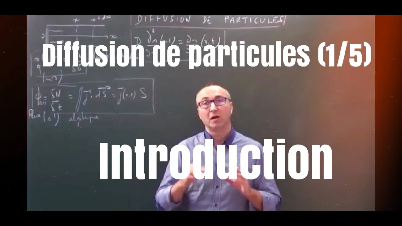
Cours diffusion de particules (1/5) : équation de diffusion de particules
80.9K
Fick's law states that flux j is proportional to the negative concentration gradient: j = -D(∂n/∂x), where D is the diffusion coefficient. The negative sign ensures flux moves from high to low concentration. Substituting Fick's law into the particle balance equation yields the standard diffusion equation: ∂n/∂t = D(∂²n/∂x²). The second derivative arises because the first derivative of flux (containing a first derivative of concentration) produces a second derivative when substituted. This equation governs how concentration profiles evolve over time in diffusive systems.
Click to watch →
Deep Dive
Fluid dynamics concepts, specifically Stokes' law for drag force acting on spherical particles in a viscous fluid.

XI Physics | Solved Numericals| Chapter No.7 |Fluid Dynamics | Part 1
73.8K
Stokes' Law states that the viscous drag force on a spherical particle falling through a viscous fluid is given by F = 6πηrv, where η is the coefficient of viscosity, r is the radius of the sphere, and v is the terminal velocity. Additionally, the terminal velocity of a spherical particle in a viscous fluid is given by v = (2/9)(ρ - σ)gr²/η, where ρ is the density of the particle, σ is the density of the fluid, g is the acceleration due to gravity, and η is the coefficient of viscosity.
Click to watch →

Stoke's law | drag force | viscosity | BS physics | class 11 physics| lecture 1 |Mechanics Mechanics
51.5K
Stokes' Law describes the drag force experienced by a spherical object moving through a viscous fluid, given by the formula F = 6πrηv, where F is the drag force, r is the radius of the sphere, η is the viscosity of the fluid, and v is the velocity of the object. The drag force depends on three factors: the radius of the sphere (larger radius means more drag), the velocity of the object (higher velocity means more drag), and the viscosity of the medium (higher viscosity means more drag). This law applies specifically to spherical objects and is valid for laminar flow conditions.
Click to watch →

MECHANICAL PROPERTIES OF FLUIDS in 1 Shot : All Concepts, Tricks & PYQs | NEET Crash Course | UMMEED
241.2K
Stokes' Law gives the viscous drag force on a sphere moving through a viscous fluid: F = 6πηrv, where η is the viscosity, r is the sphere radius, and v is the velocity. This law applies for small spheres moving slowly through viscous fluids (low Reynolds number). The force is proportional to the radius, velocity, and viscosity.
Click to watch →

IMPORTANT DERIVATIONS 🔥CLASS 11TH PHYSICS FROM BOOK 2 || MUNIL SIR
180.1K
Stokes' Law describes the viscous drag force experienced by a spherical object moving through a viscous fluid. The drag force is given by F = 6πrηv, where r is the radius of the sphere, η is the coefficient of viscosity (also called coefficient of friction), and v is the velocity of the sphere. The coefficient of viscosity measures the fluid's resistance to flow - higher viscosity means more resistance (like honey or mud). This law applies to laminar flow conditions where the Reynolds number is low.
Click to watch →

Drag Force & Stokes’ Law | Fluid Dynamics Explained | Class 11 Physics Chapter 6 | DEAR CONCEPT
390
Stokes' Law states that the drag force on a spherical object is given by: FD = 6π η R V, where η is the coefficient of viscosity, R is the radius of the sphere, and V is the velocity of the object. This formula shows that drag force is directly proportional to viscosity, radius, and velocity.
Click to watch →
Deep Dive
Basic probability and statistics, particularly the mathematical concept of a random walk and mean squared displacement.
Probability and Statistics (Module 1.9 - English)
435
Random walks model particles taking steps of fixed length in random directions. In one dimension, a walker moves +1 or -1 with probabilities p and q (p+q=1). The binomial distribution P(k) = C(n,k)p^kq^(n-k) gives the probability of k right steps in n trials. For symmetric walks (p=q=½), average displacement is zero but mean squared displacement equals n, growing as √n. This applies to atomic motion in gases, stock markets, and polymer chains. Mathematically, random walks use independent identically distributed random variables X₁,X₂,...,Xₙ where each Xᵢ = ±1 with probability ½. The position after n steps is Sₙ = ΣXᵢ. For symmetric walks, the probability of returning to origin after 2m steps is P(2m) = C(2m,m)(½)^(2m). First return requires never touching the origin before step 2m, excluding paths that cross the origin multiple times.
Click to watch →

Theory of random walk : Mean squared displacement
2.8K
This section establishes the theoretical foundation of random walk in particle systems. It begins by defining random walk as the motion of particles in liquids and gases where particles move in straight lines until colliding, then change direction randomly. The net displacement after n jumps is the vector sum of individual jump vectors. In systems of many particles, each moves randomly in all directions with independent jump directions and magnitudes, causing isotropic spreading. However, average net displacement is zero due to cancellation between positive and negative displacements. Einstein established that mean square displacement (MSD), denoted ⟨r²⟩, is the correct parameter to measure particle distribution spreading. Mathematically, MSD expands to include diagonal terms (squares of individual jumps) and off-diagonal terms (dot products between different jumps), requiring careful summation over all pairs.
Click to watch →

EC 303 class 1 - Stochastic and Spatial Dynamics in Biology
405
This extensive section develops random walk theory from probability fundamentals to practical applications. The instructor explains independence (one outcome doesn't affect another), covariance and correlation (measuring how variables vary together), and identically distributed variables (sharing the same probability distribution). Combined with independence, this gives the i.i.d. assumption fundamental to random walk models. For an unbiased random walk starting at the origin, the mean displacement <x(t)> = 0 because at each step, the expected change is zero. Two-dimensional random walks can be simulated by choosing random step lengths in both x and y directions. Mean Square Displacement (MSD) captures the actual spread of trajectories by averaging squared displacement from the origin: MSD(t) = <(x(t) - x(0))²>. Unlike mean displacement, MSD cannot be zero and provides a meaningful measure of how far organisms have moved from their starting point.
Click to watch →

Brownian motion random walks and coin flips
143
The probability distribution f_N(n) describes likelihood of being at displacement n after N steps. For small step counts, all outcomes can be enumerated: 0 steps yields 100% at origin; 1 step yields 50% at ±1; 2 steps yield 25% at ±2 and 50% at 0; 3 steps yield 12.5% at ±3, 37.5% at ±1, and 12.5% at 0. These probabilities follow binomial coefficients and correspond to Pascal's triangle rows, where each entry equals the sum of two diagonal entries above it. The coefficient for k heads in N steps is C(N, k) = N!/(k!(N-k)!), representing the number of paths leading to that outcome. In unbiased random walks, the mean displacement from origin is always zero because left and right movements cancel symmetrically. However, the mean squared displacement equals the number of steps taken, because squaring eliminates sign differences. This relationship—mean squared displacement equals time—is a fundamental property of diffusion processes.
Click to watch →

Probabilità, Statistica e Random Walk! | The Feynman Club 6
1.9K
A random walk is a model where an object moves in discrete steps with random directions. In a symmetric random walk (equal left/right probability), the mean position after n steps is zero because for every path to +d, there's a symmetric path to -d. The mean squared displacement after n steps is exactly n, derived by considering how squared displacement changes with each step. The root mean squared displacement (RMSD) is √n, representing the typical distance from the origin. This growth as √n, not linearly with n, is a key property of random walks.
Click to watch →
Prerequisite Knowledge
- Concept 01Fundamentals of the kinetic theory of gases, including thermal energy (kT) and molecular collisions.
- Concept 02Fick's laws of diffusion, which describe how concentration gradients drive macroscopic particle flux.
- Concept 03Fluid dynamics concepts, specifically Stokes' law for drag force acting on spherical particles in a viscous fluid.
- Concept 04Basic probability and statistics, particularly the mathematical concept of a random walk and mean squared displacement.
Subsequent Learning
- Step 01The Langevin Equation, which introduces stochastic differential equations to model random forces on a particle.
- Step 02The Fokker-Planck Equation, used to describe the time evolution of the probability density function for position and velocity.
- Step 03The Fluctuation-Dissipation Theorem, which generalizes the link between thermal fluctuations and dissipative systems.
- Step 04Jean Perrin's experimental work on Brownian motion, which validated Einstein's theory and helped prove the physical existence of atoms.
Course Start
Einstein's Theory
Model Cylinder
Particle Flow
Flux Equation
Diffusion Relation
Course Start
0:01Playing Section
- 1
Lecture begins with greetings.
- 2
Sets up physics topic.
- 3
Introduces Brownian motion.
The Langevin Equation and the Short-Time Ballistic Limit
While Einstein’s theory of Brownian motion successfully proved the existence of atoms by treating particle movement as a diffusion process, it has notable physical limitations. Einstein’s derivation assumes the fluid is a continuous medium and neglects the inertia of the Brownian particle, implying infinite instantaneous velocity at infinitesimally small time steps. To address these shortcomings, Paul Langevin in 1908 introduced a stochastic approach incorporating Newton's second law with a random fluctuating force. This was later mathematically refined as the Ornstein-Uhlenbeck process. This alternative perspective reveals that at extremely short time scales (the ballistic regime), a particle's displacement is proportional to time rather than the square root of time, meaning it behaves like a free inertial particle before collisions randomize its path. Understanding this limit is vital for modern high-resolution physics experiments that measure particle dynamics at microsecond scales.
Deep Dive
The Langevin Equation, which introduces stochastic differential equations to model random forces on a particle.

Introduction to Ito Calculus
2.2K
The Langevin equation models physical systems subject to both deterministic forces and random fluctuations. For a large particle in a fluid, the equation is m(dv/dt) = -γv + F_rand, where -γv represents damping from collisions and F_rand is a random force modeling unpredictable impacts. The random force is formally defined as white noise, the derivative of Brownian motion: C(t) = dB/dt, with zero mean and delta-correlated in time. This leads to stochastic differential equations (SDEs) of the form dX = μ(X,t)dt + σ(X,t)dB, which are always understood in integral form. The Langevin equation thus provides a physically motivated starting point for understanding stochastic calculus and its applications in physics and finance.
Click to watch →
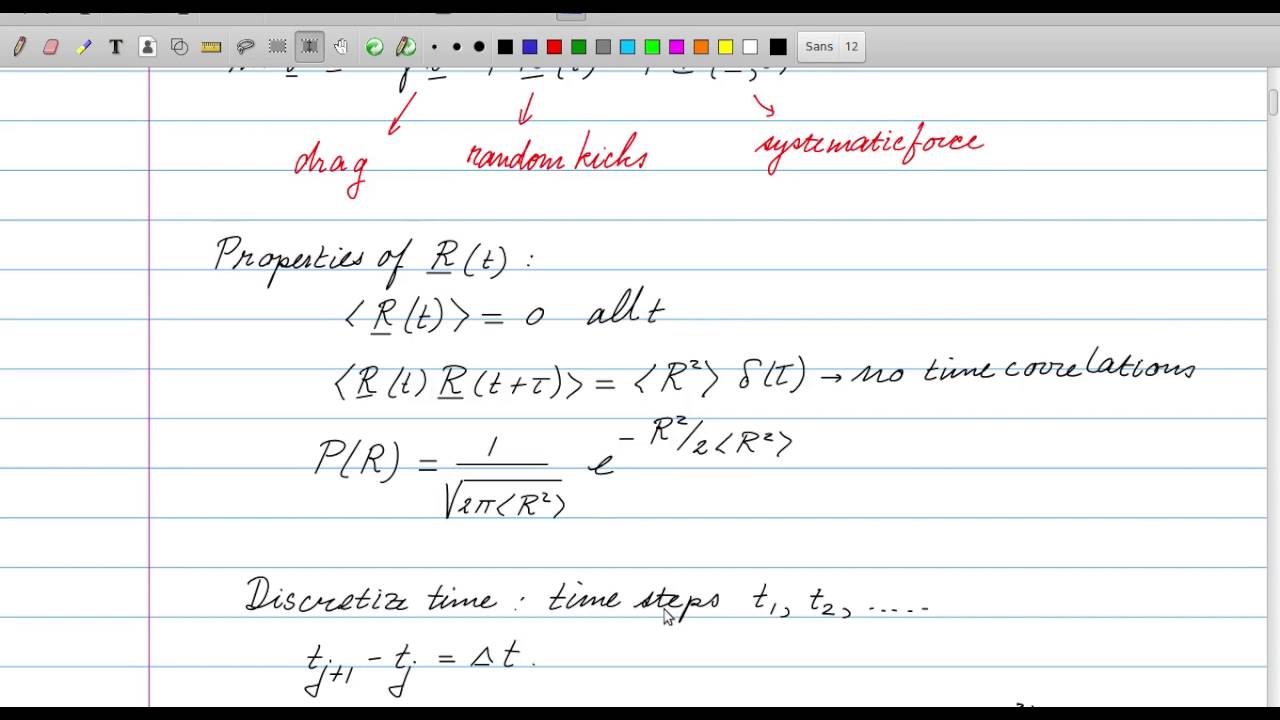
fluctuations and the Langevin equation
6.9K
The Langevin equation (m dv/dt = -γv + R + f) describes particle motion under drag, random forces, and systematic forces, where the random force R has zero mean, no time correlations, and Gaussian statistics; solving this equation leads to the Fokker-Planck equation governing probability distributions, which yields the diffusion equation (∂P/∂t = D ∂²P/∂x²) showing that mean squared displacement grows linearly with time (⟨x²⟩ = 4Dt), with the diffusion constant D = kBT/γ connecting microscopic random forces to macroscopic transport phenomena through the Einstein relation.
Click to watch →
Lecture 0 Part III: Deriving the Langevin Equation
6.4K
The Langevin equation describes the motion of a single particle in a fluid by accounting for three types of forces: fluid drag (proportional to velocity, given by Stokes' law γ = 6πηR/M for spherical particles), deterministic forces (such as electric fields, gravity, or molecular bonds), and random molecular forces from collisions with surrounding fluid molecules; the equation is written as M(dv/dt) = -Mγv + F_deterministic + M·RT, where RT represents random forces proportional to √T, enabling the study of both equilibrium properties and dynamic behavior of particles at microscopic scales.
Click to watch →
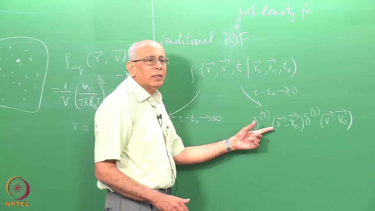
Mod-01 Lec-02 The Langevin model (Part 1)
39.4K
The Langevin model describes the motion of a large particle (Brownian particle) in a fluid by incorporating both deterministic viscous drag and random collision forces, leading to the equation m(dv/dt) = -γv + η(t), where γ represents the friction coefficient and η(t) is Gaussian white noise; this model resolves the unphysical energy increase problem of the original Langevin equation by accounting for the particle's velocity-dependent drag force that dissipates energy, allowing the system to reach thermal equilibrium with finite energy.
Click to watch →

Langevin and Fokker Planck equations
28.1K
The Langevin equation describes the motion of heavy particles (like smoke particles or solute molecules) surrounded by light particles, incorporating both a frictional force (-γV) and a random force to capture collision effects; by analyzing the statistical properties of the random force (zero mean, uncorrelated at different times, Gaussian distribution) and deriving the corresponding Fokker-Planck equation for the velocity distribution, we find that the system evolves toward the Maxwell-Boltzmann distribution, with the fluctuation-dissipation theorem relating the random force strength to temperature and friction coefficient (Q = 2γkBT).
Click to watch →
Deep Dive
The Fokker-Planck Equation, used to describe the time evolution of the probability density function for position and velocity.

Fokker-Planck Equation
14.3K
The Fokker-Planck equation describes the time evolution of the probability density function P(x,t|y) for a stochastic process defined by dX = B(X)dt + σdW, where B is the drift coefficient and σ is the diffusion coefficient. Using Ito's calculus, the equation is derived as ∂P/∂t = L[P], where the generator operator L = (1/2)∇·(σσ^T∇) - ∇·(B). Two types of boundary conditions are discussed: reflecting boundary conditions require zero probability flux (J·n = 0), while absorbing boundary conditions set P = 0 on the boundary.
Click to watch →

Aula 15.2 - A equação de Fokker-Planck
593
The Fokker-Planck equation describes the time evolution of the probability density function for a stochastic process, derived from the limit of a symmetric random walk where the expected value remains constant and the variance increases linearly with time, leading to a diffusion equation that models how probability distributions spread out over time.
Click to watch →

Fokker Plank Equation | Statistical Mechanics | Prof Kirti Gangrade
18.5K
The Fokker-Planck equation is a partial differential equation that describes the time evolution of the probability distribution function of the velocity of a particle, and more generally, the time evolution of the probability distribution of any stochastic process. It is derived from the Langevin equation and provides a mathematical framework for understanding how systems evolve under the influence of random forces and damping, making it essential for studying Brownian motion and other diffusive processes in statistical mechanics.
Click to watch →
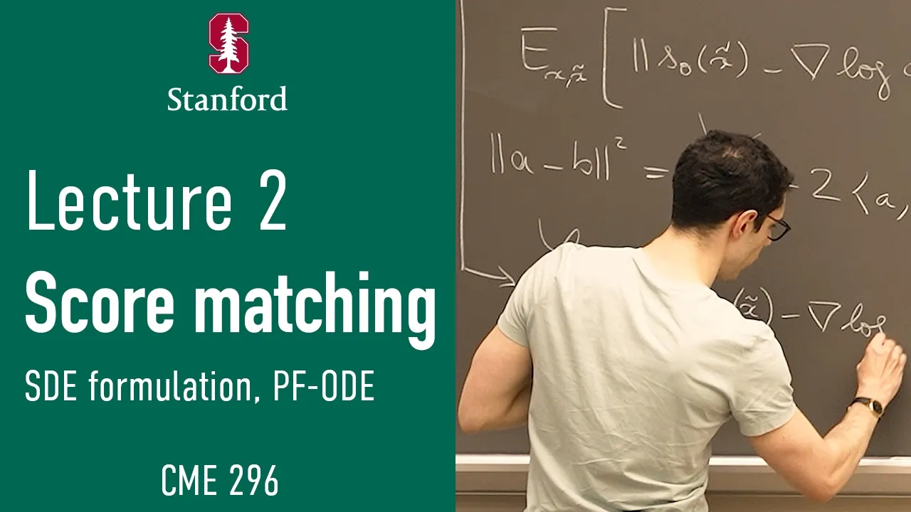
Stanford CME296 Diffusion & Large Vision Models | Spring 2026 | Lecture 2 - Score matching
662
The Fokker-Planck equation describes probability density evolution under SDE: ∂P/∂t = -∇·(fP) + ½g²∇²P. The first term represents deterministic advection, the second represents stochastic spreading. The Probability Flow ODE is derived by rearranging this equation and using the velocity field V(x,t) = f(x,t) - ½g(t)²∇log P(x,t). This ODE preserves the same probability flow as the SDE but is deterministic, enabling more efficient sampling with adaptive step sizes. The PF-ODE and SDE produce the same final distribution but have different trajectories.
Click to watch →
Solución numérica de ecuaciones diferenciales estocásticas
260
The Fokker-Planck equation describes the time evolution of probability density functions for stochastic processes. It is a partial differential equation that translates stochastic problems into deterministic ones. For dX = f(X,t)dt + g(X,t)dW, the corresponding Fokker-Planck equation is ∂p/∂t = -∂(fp)/∂x + (1/2)∂²( g²p)/∂x². For geometric Brownian motion with dX = μX dt + σX dW, the solution is log-normal: p(x,t) = (1/(xσ√(2πt))) exp(-(ln(x/x₀) - (μ-σ²/2)t)²/(2σ²t)). This equation is fundamental for modeling financial assets and other phenomena with multiplicative noise.
Click to watch →
Deep Dive
The Fluctuation-Dissipation Theorem, which generalizes the link between thermal fluctuations and dissipative systems.

Lecture 50 : Fluctutaion Dissipation Theorem
151
The Fluctuation-Dissipation Theorem establishes a fundamental relationship between the correlation function (describing thermal fluctuations in equilibrium systems) and the Green's function (describing the system's response to external perturbations), stating that they are proportional with the proportionality constant being 2kBT/ω, where kB is Boltzmann's constant, T is temperature, and ω is the frequency; this theorem applies only to systems near equilibrium and connects microscopic dissipation mechanisms to macroscopic thermal fluctuations.
Click to watch →
What Is Fluctuation-dissipation Theorem? - Physics Frontier
568
The fluctuation-dissipation theorem is a fundamental principle in physics that establishes a direct relationship between the natural random fluctuations occurring in a system at equilibrium and its response to external disturbances, specifically showing that how a system loses energy when pushed out of equilibrium is determined by its spontaneous fluctuations; mathematically, this connects the correlation function of fluctuations to the imaginary part of the system's susceptibility, with applications ranging from analyzing noise in electronic circuits to understanding Brownian motion and polymer behavior.
Click to watch →
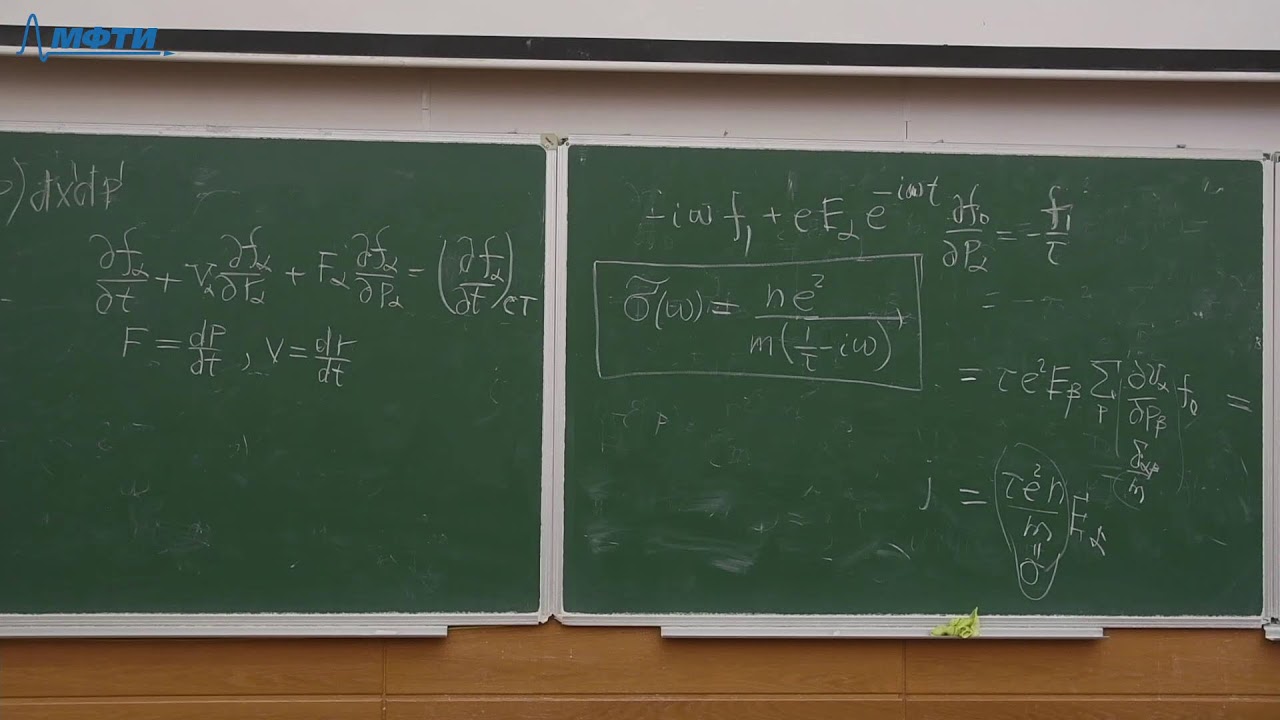
Физическая кинетика, С.В. Панюков, 2 лекция, 09.02.2024
1.1K
The fluctuation-dissipation theorem establishes that any dissipative system element (such as an electrical resistor) simultaneously generates random thermal fluctuations (Nyquist noise) described by the formula ⟨U²⟩ = 4kTΔν/R, where the mean square voltage is proportional to temperature, frequency interval, and inversely proportional to resistance. This theorem connects the response of a system to external perturbations with its intrinsic thermal fluctuations, showing that dissipation and fluctuations are two manifestations of the same underlying physics.
Click to watch →
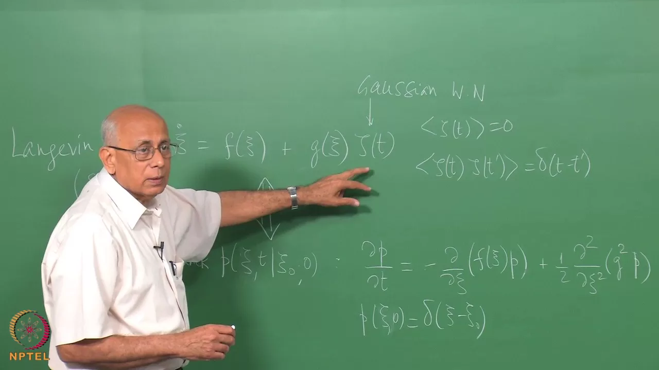
Mod-01 Lec-17 Fokker-Planck equations (Part 1)
24.5K
The fluctuation-dissipation theorem establishes that for thermal equilibrium to be maintained, the dissipation coefficient γ and noise strength must satisfy γ = 2mγkBT/m, where kBT is the thermal energy. This ensures that the equilibrium distribution obtained from the Fokker-Planck equation matches the Maxwell-Boltzmann distribution. Without this relationship, the system would not reach thermal equilibrium when averaged over all noise realizations.
Click to watch →

Консультация к письменному экзамену по термодинамике от Леши Свинцицкого, 07.06.2023
5.9K
The fluctuation-dissipation theorem relates the fluctuations in a system to its response to external perturbations. For an ideal gas, the relative fluctuation of the number of particles in a subvolume is 1/√N, where N is the average number of particles. This is derived from the fact that the variance of the number of particles equals the mean (for an ideal gas), so the standard deviation is √N and the relative fluctuation is 1/√N. This result is fundamental to understanding why macroscopic systems appear deterministic despite being composed of many fluctuating microscopic components.
Click to watch →
Deep Dive
Jean Perrin's experimental work on Brownian motion, which validated Einstein's theory and helped prove the physical existence of atoms.

Einstein theory of Brownian motion and determination of Avogadro's number by Perrin.
1.1K
Jean Baptiste Perrin experimentally verified Einstein's theory by measuring Brownian motion. Using high-power microscopes with eyepiece scales, he observed individual particles at 30-second intervals, plotting their zigzag paths. By calculating mean square displacement from displacement vectors and substituting into the theoretical formula N = (RT)/(<r²> × 3πηa × t), he determined Avogadro's number experimentally. His result (≈6.82 × 10²³) closely matched accepted values, confirming Einstein's theory and providing direct evidence for atomic existence.
Click to watch →
![[統計力學特論] 14、Brownian Motion](https://i.ytimg.com/vi_webp/hm5SzeGLaLE/maxresdefault.webp)
[統計力學特論] 14、Brownian Motion
2.4K
Jean Baptiste Perrin experimentally verified Einstein's theory by measuring Avogadro's number. He tracked individual pollen particles undergoing Brownian motion, measured their terminal velocity to determine mobility μ using Stokes' law, and measured the diffusion coefficient D. Using the Einstein relation D = kTμ, he calculated Avogadro's number N_A = 6πaηRT/D. His result of approximately 7×10²³ molecules per mole provided direct experimental evidence for atomic existence, earning him the Nobel Prize in 1926. This demonstrated that atoms are real physical entities whose existence could be confirmed through precise measurements of microscopic phenomena.
Click to watch →

Перрен, Жан Батист
361
Jean-Baptiste Perrin, a French physicist who received the 1926 Nobel Prize in Physics, experimentally verified Einstein's theoretical work on Brownian motion, providing definitive proof of the existence of atoms and molecules by demonstrating that the random motion of particles in fluids is caused by molecular collisions, thus ending a century-long debate about atomic theory.
Click to watch →

The Physicist That Validated the Existence of Atoms
9.6K
Jean Baptiste Perrin's 1909 experiments confirmed Einstein's 1905 theory that Brownian motion results from collisions between water molecules and suspended particles, providing experimental evidence for the atomic nature of matter by calculating Avogadro's number and thereby resolving the century-old debate between atomism and energetics.
Click to watch →

Jean Perrin - Il a mis tout le monde d'accord - LPPV 12
244.6K
Jean Perrin (1870-1948) was a French physicist who experimentally proved the existence of atoms by verifying Einstein's predictions on Brownian motion and determining Avogadro's number through multiple independent methods, including diffusion of Rayleigh, critical opalescence, and radioactive decay experiments, which convinced the scientific community of atomic reality.
Click to watch →
Course Start
Einstein's Theory
Model Cylinder
Particle Flow
Flux Equation
Diffusion Relation
Course Start
0:01- 1
Lecture begins with greetings.
- 2
Sets up physics topic.
- 3
Introduces Brownian motion.
The Langevin Equation and the Short-Time Ballistic Limit
While Einstein’s theory of Brownian motion successfully proved the existence of atoms by treating particle movement as a diffusion process, it has notable physical limitations. Einstein’s derivation assumes the fluid is a continuous medium and neglects the inertia of the Brownian particle, implying infinite instantaneous velocity at infinitesimally small time steps. To address these shortcomings, Paul Langevin in 1908 introduced a stochastic approach incorporating Newton's second law with a random fluctuating force. This was later mathematically refined as the Ornstein-Uhlenbeck process. This alternative perspective reveals that at extremely short time scales (the ballistic regime), a particle's displacement is proportional to time rather than the square root of time, meaning it behaves like a free inertial particle before collisions randomize its path. Understanding this limit is vital for modern high-resolution physics experiments that measure particle dynamics at microsecond scales.
Fundamentals of the kinetic theory of gases, including thermal energy (kT) and molecular collisions.
Fick's laws of diffusion, which describe how concentration gradients drive macroscopic particle flux.
Fluid dynamics concepts, specifically Stokes' law for drag force acting on spherical particles in a viscous fluid.
Basic probability and statistics, particularly the mathematical concept of a random walk and mean squared displacement.
The Langevin Equation, which introduces stochastic differential equations to model random forces on a particle.
The Fokker-Planck Equation, used to describe the time evolution of the probability density function for position and velocity.
The Fluctuation-Dissipation Theorem, which generalizes the link between thermal fluctuations and dissipative systems.
Jean Perrin's experimental work on Brownian motion, which validated Einstein's theory and helped prove the physical existence of atoms.
44.1K views885likes16:38@pankajphysicsgulatiOriginal Release: 2021-08-08
[Music] hello students how are you welcome to my youtube foreign einstein formulated a quantitative theory for the brownian motion of the on the basis of the fact that the brown and particles tend to diffuse into the medium on in osmotic pressure between different parts due to difference in concentration of the suspended particle which give rise let us consider an imagery cylinder in the medium with its axis parallel to the x-axis or is cylindrical x-axis k parallel hogi means this line represents your x-axis let a be the cross-sectional area of end surfaces s1 and s2 surfaces let delta is equal to distance between n surfaces s one and s two in don't know and surfaces molecular concentration is the excess of molecules crossing middle [Music] excess of molecules crossing the middle layer as to the right that will be equal to half is n1 minus n2 molecules crossing the middle layer as to the right per unit area per second that will be equal to that will be equal to half delta square dn by dx square divided by area into time say s is is diffusion coefficient [Music] comparing 3 and 4 we get 1 by 2 del square t by t d n by dx that will be equal to d d n by d x so d n by d x d n by d x cancels till then take care
Up Next

92:17
Fundamental Forces in Soft Matter Physics | Lecture 1
@ICAMI2CAMpresentations
776 views•2016-07-07

12:53
21cm Hyperfine Transition in Neutral Hydrogen: Radio Astronomy Basics
@AaronRobertParsons
12.4K views•2011-10-13

9:12
Meissner Effect in Superconductors Explained with Proof
@pankajphysicsgulati
259.6K views•2019-01-14

27:14
Entropy and the Second Law of Thermodynamics Explained
@veritasium
27.5M views•2023-07-01
Related Study Plans & Knowledge Roadmaps
Structured learning paths in Physics
physics
Nuclear Physics (Decay, Fission & Reactors)
01Atomic Structure and the Binding Force
02Radioactive Decay and Half-Life
03Nuclear Fission Mechanics and Chain Reactions
+ 2 more learning modules
12h5 modules
Explore Roadmap
physics
Soft Matter (Polymers, Colloids & Rheology)
01Foundations of Soft Matter & Thermal Forces
02Polymer Physics and Macromolecules
03Colloids, Surfactants, and Self-Assembly
+ 2 more learning modules
38h5 modules
Explore Roadmap
physics
Analytical Mechanics: Lagrangian & Hamiltonian
01Mathematical Foundations: Calculus of Variations
02From Newtonian Mechanics to Constraint Dynamics
03The Principle of Least Action & Lagrangian Mechanics
+ 3 more learning modules
28h6 modules
Explore Roadmap
physics
General Relativity (Spacetime & Cosmology)
01Foundations of Relativity: Special Relativity
02The Geometry of Spacetime: Equivalence Principle & Curvature
03Einstein's Field Equations: The Mathematics of Gravity
+ 2 more learning modules
55h5 modules
Explore Roadmap