














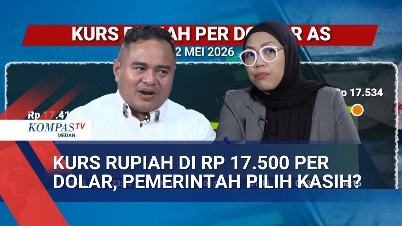









The IS-LM-BP model extends the basic IS-LM framework to open economies by incorporating the balance of payments (BP) curve, which shows equilibrium in the current account (net exports) and capital account; the BP curve's steepness relative to the LM curve determines whether expansionary fiscal or monetary policy leads to balance of payments deficits or surpluses, with steeper BP curves resulting in deficits from fiscal expansion and flatter BP curves resulting in surplus improvements.
IS-LM-BP Model: Open Economy Macroeconomics Tutorial
Added:The Closed-Economy IS-LM Model: Understanding goods market equilibrium (IS curve) and money market equilibrium (LM curve) in a closed setting.
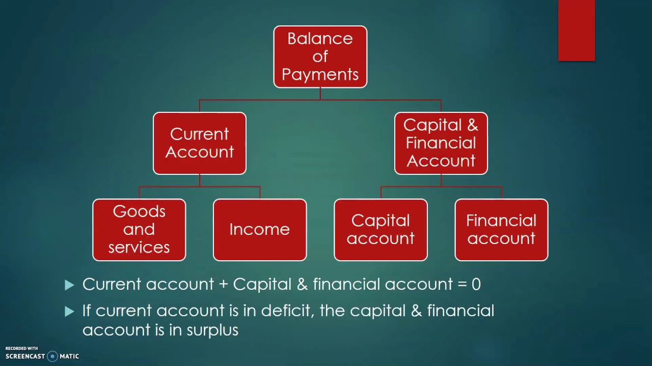
Balance of Payments (BoP) Accounting: Familiarity with the current account, capital/financial account, and how international transactions are recorded.
Exchange Rate Regimes: Clear distinction between fixed and floating exchange rate systems and their basic operational mechanics.
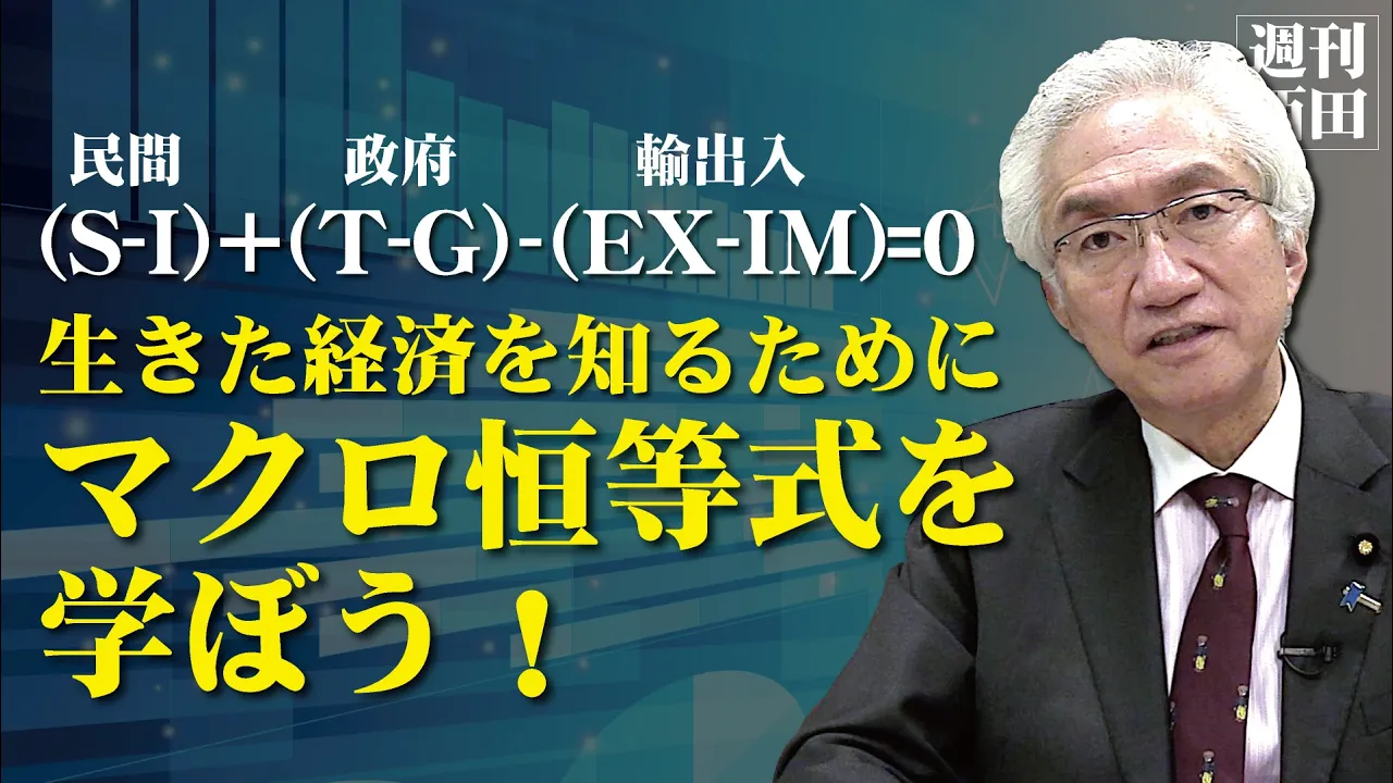
Basic Open Economy Macroeconomic Identities: Understanding the role of net exports (NX) and net capital outflows in national income accounting.
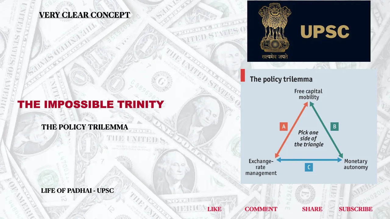
The Policy Trilemma (Impossible Trinity): Exploring the trade-offs between fixed exchange rates, free capital mobility, and independent monetary policy.
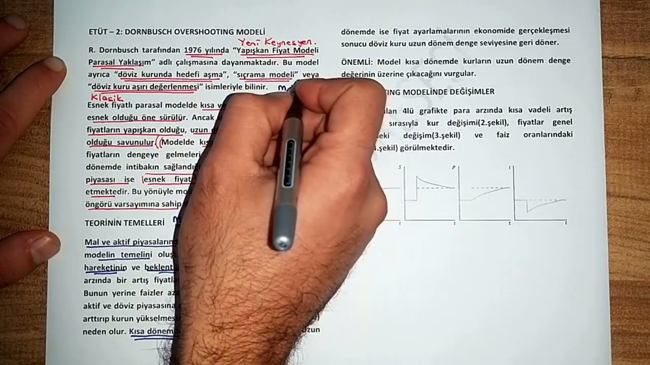
The Dornbusch Overshooting Model: Analyzing exchange rate volatility and adjustment mechanisms in the short run when prices are sticky.
Open Economy AD-AS Framework: Transitioning from short-run IS-LM-BP analysis to a medium-run model where price levels are flexible.
Historical Currency Crises: Applying the IS-LM-BP framework to analyze real-world events, such as the 1997 Asian Financial Crisis or Eurozone structural issues.
41.3K views207likes16:55Original Release: 2015-03-20
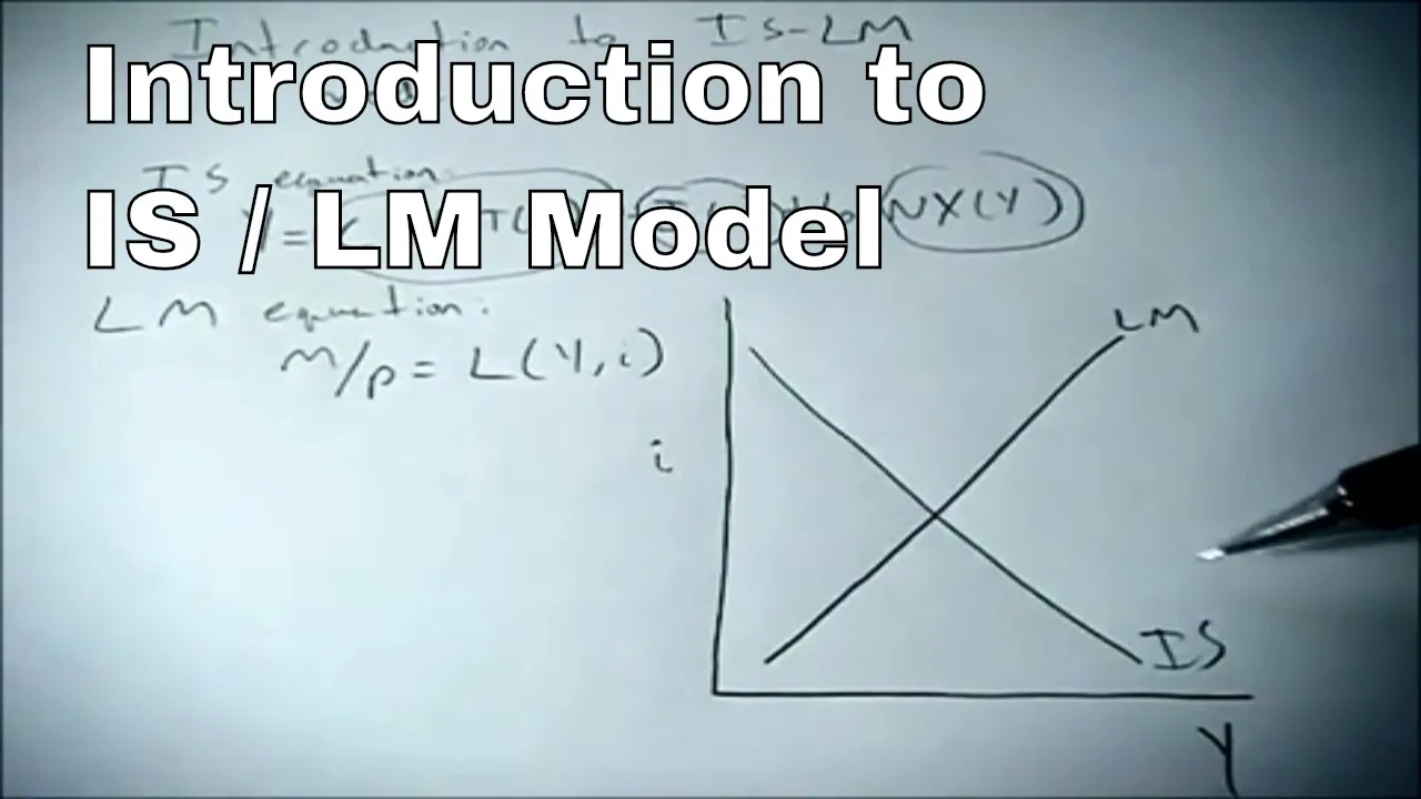
The IS-LM model is a two sector model of the macro economy. It is macroeconomics' attempt to create a general equilibrium model. In this simple model, there are two sectors represented by two equations. The first equation represents the real output sector - often called the IS equation, and the second equation represents the monetary sector or financial sector. There are two unknown variables in this system, or two variables to determine: output and interest rates - Y & i There are two policy variables in the system: G, the level of government spending, and M the level of the money supply. The price level can be an endogenous variable in the system, and we will then have three endogenous variables in a two equation system, which cannot be solved uniquely. However, we can make one of these three endogenous variables relatively exogenous, and we are back to a two equation system. The real output sector is usually represented by the national income accounting identity at a first pass: Y = C + I + G, and that says that on the left hand side, the output that is produced is distributed across three sectors - or is used by three sectors: the consumption sector, the investment sector, and the government sector. Said differently, there are three main users of the goods that are produced in the economy: the government, households, and firms. Equation 2 is the equilibrium of money supply and money demand in real terms. So on the right hand side, we have the demand for money which is a positive function of output and a negative function of the interest rate. Because our model is linearized, we see the coefficients L1 and L2, but in a general functional form notation, we'd say M is a function of y (positive) and i (negative). The linearization helps to make the arithmetic simpler. On the left-hand side of equation 2, we have the real money supply- which is the nominal money supply M divided by the price level. If we allow the prices to be held relatively constant, then the left-hand side of equation 2 is a constant and we have a two-equation system, with two unknown variables: interest rate and output. If prices are allowed to be endogenous, we have three endogenous variables and two equations so there's no unique solution to this system. This has created a very interesting set of possibilities and in order to get a unique solution for the system, various theories have chosen to make Y relatively constant - that's the classical theory, or make P constant - that's the Keynesian theory, and that's how we find a unique solution to this system. This problem has been resolved in elementary macroeconomics textbooks by making one of the three variables relatively constant. The two easy alternatives are the Keynesian assumption of constant prices, and the classical assumption of constant output. And what we mean is that the two equation system does not determine prices for the Keynesians, nor does it determine output for the classicists. From that perspective then, the variables are not exogenous per se, but relatively exogenous: they are determined outside of the system that we are showing. Note that the classical model yields a recursive solution where interest rates are determined solely in the output market, leaving prices to be determined by monetary forces. Indeed, if nothing changes in the real sector, then an increase in the money supply will result only in an increase in prices. This is often summarized as money causes inflation or money is a veil. Monetary policy is therefore not an effective policy tool for the classicists except to fight inflation. The classical model is said to be representative of the long run, since it is possible to obtain real effects of expansionary fiscal and monetary policy in the short run, but these will not be sustained once everyone is fully informed in the long run.
We are interested in a graphical representation of this analysis, and first we will start by deriving the IS curve to give you a sense as to where it came from. The IS curve, which is the equilibrium in the real sector, comes from two main ideas: that investment is a function of interest rates (negative), this is the top left-hand panel and that saving is a positive function of output.
The third assumption in this sector is that domestic savings equal domestic investment, and when we put these variables together in our system, we get the IS curve - and I will show you how that is derived. In the monetary sector we derive the LM curve - again based on the same types of ideas: that the speculative demand for money is an inverse function of the interest rate, and the transactions demand for money is a positive function of output. We have an adding up equation which says the supply of money is the sum of the transactions demand and the speculative demand at equilibrium, so there are two uses for money - two reasons individuals are holding money here: for transactions purposes and for speculative purposes, and when we combine this information together, we trade so what is known as the LM curve.
The LM curve will be a positive relationship showing equilibrium in the money market, and the positive relationship will say as Y increases in order to preserve equilibrium, I needs to increase. The interest rate and the output levels will be positively correlated at equilibrium in the money market. In tracing out the IS curve, we will obtain an inverse relationship between interest rates and output at equilibrium. That says that in order to preserve equilibrium in the real sector, increases in output will generally be correlated with decreases in the interest rate. So here we have the traced out IS curve - inverse correlation between I and y at equilibrium in the real sector, and the LM curve a positive correlation of I and Y in the monetary sector. When our two equation system is put together to identify some unique equilibrium, we get the IS curve and the LM curve in the same panel I against Y, and we can find one unique equilibrium of interest rates and output. We now move on to discuss policy consequences, and the two policies we are going to focus on are expansionary fiscal policy and expansionary monetary policy.
Expansionary fiscal policy shifts the IS curve to the right.
Intuitively we are saying that ceteris paribus, if we were to increase the level of government spending, holding the interest rates constant, we would expect the expansionary fiscal policy to grow the economy: increases in Y for every level of I holding the level of I constant then we're expecting every point on the Y panel to be to the right and as we trace of all of the expansions here we're going to see the entire IS curve shifting to the right. Notice that traces out an equilibrium that is a higher level of interest rate on the vertical axis and a higher level of output on the horizontal axis.
Expansionary fiscal policy yields a higher interest rate and a higher output level. Let us move to the LM curve. We will do the same type of experiment.
So we ask the question what happens if we were to increase the money supply, while holding the interest rate constant? To preserve the equilibrium, increase on the supply side needs to lead to an increase on the demand side, and if the interest rate is held constant, that translates into an increase in output.
An alternative way of asking the same question is: for output held constant, what does an increase in the money supply do to the interest rate? An increase in the supply of money will, ceteris paribus, lead to a lower interest rate, because we flooded the market with local currency, and the only way individuals will borrow this extra money is at a lower opportunity cost price or lower interest rate. We understand then that the LM curve will shift to the right if there's expansionary monetary policy. We will get increases in output and a decrease in the interest rate. We now introduce the idea of the balance of payments equilibrium or the BP curve. We define balance of payments as net exports (or the current account) plus the capital and financial account. I use upper-case KA to represent that account. And we are going to identify equilibrium in the balance of payments which means that there is no balance of payment surplus or deficit - the balance of payments will be in equilibrium, and net exports will be defined as a positive function of the exchange rate and a negative function of output, so we are saying that if foreign currency were to increase in price it would mean that domestic currency is relatively cheaper, therefore domestic goods are relatively cheaper and therefore exports might increase. On the demand side, however, if foreign currency is more expensive, than foreign goods are more expensive; so the demand for foreign goods will decline, and because our net exports is exports minus imports, a decline in imports is an improvement in the balance of trade, and that is why we say an increase in E will lead to an increase in net exports. An increase in domestic income will lead to more imports. The reason that we have a negative correlation between net exports and income is because imports will increase, ceteris paribus. That means that the trade balance will worsen. Net exports will decline when income increases so we have signed the two variables in the net exports equation and we assumed that the capital and financial account is dependent on the spread between domestic interest rates and foreign interest rates. Ceteris paribus, a higher domestic interest rate will bring more money into the domestic economy more foreign money into the domestic economy and improve the capital account. Remember that our graphical analysis shows income and interest rates on the axes so we want to trace out what the BP curve would look like in this panel of I against Y.
So we're going to hold E relatively constant, and ask how can the balance of payments remain in equilibrium?So if I were to increase, the capital account would improve, and in order for the balance of payments to remain in balance at zero, it means that the current account needs to worsen. This manifests itself in a higher income or output higher income will mean that we import more, and, ceteris paribus, that will lead to a decline or deterioration of net exports. So we get a positive correlation between domestic interest rates and domestic income or output, and this creates a very interesting analysis.
Note that every point in the panel here has a meaning, and this is something that's a little different than we've considered before - we've generally considered equilibrium points, but I want to consider all of the disequilibrium points in the panel as well. So a point A or B, which is north or west of the balance of payment equilibrium equation would represent either a higher level of interest rate or a lower level of output when compared to the equilibrium.
A higher interest rate should cause the capital account to improve ceteris paribus, so for a given level of output, a higher interest rate will cause the balance of payments to go into surplus. Alternatively, a lower level of income will cause imports to go down, and the balance of trade should improve. And now we're going to have the same effect. So we have an increase in interest rate leading to an improvement in the capital and financial account or alternatively a decline in income leading to an improvement in the current account.
So any point in the space to the north or west of the balance of payments equilibrium line will be a balance of payment surplus: A and B then represent points of surplus in the balance of payments. Note that the higher is interest rate or the lower is income the greater will be that surplus. So the farther away we are from the BP line, the larger is the surplus in the balance of payments. It should not be surprising that points to the right of the balance of payments equation will represent deficits in the overall balance of payments: higher income leads to more imports, ceteris paribus. That worsens the trade balance and ceteris paribus that worsens the balance of payments.
Alternatively we can say lower interest rates domestically cause a net outflow in the capital account: ceteris paribus a lower interest rate will yield an outflow in the net position of the capital account, and that will worsen the overall balance of payments. So points C and D will reflect the overall balance of payments being in deficit.
The analysis is extremely interesting here now because we have two positive slopes and one negative slope. The crux of the analysis will be: which of the two positively sloped curves is steeper?
We will come to the conclusion that when the balance of payments curve is steeper of the two, expansionary fiscal policy will lead to a balance of payments deficit.
When the balance of payments is flatter than the LM curve, expansionary fiscal policy will lead to an improvement in the overall balance of payments.
The steepness of the BP curve then matters a lot to the analysis.
This is the most interesting part of IS LM BP analysis, and hopefully the intuition will make sense. So we really want to ask the question: what is the consequence of expansionary fiscal and monetary policy, and do we get inconsistent results for the balance of payments? Our question then ultimately is: what is the impact of expansionary fiscal or monetary policy on their balance of payments? All of the other questions retain their sign and this one becomes interesting because we get opposite signs. At the end of the day, we want to ask the question: what causes the balance of payments curve to be either steeper than the LM curve or flatter than the LM curve what causes the balance of payments equation to be relatively steep? What causes the balance of payments equation to be relatively flat? This will have consequences for the impact of expansionary fiscal policy on the country's balance of payments. Notice that this is a short run phenomenon, so we should not exhaust too much effort on answering this question. Just note that there's an interesting policy difference based on the steepness of the BP curve. In order to simplify the answers to the question, we're going to work with two extreme cases of a vertical BP curve and a horizontal BP curve. Most textbooks show the horizontal BP curve, and I like the vertical BP curve because it speaks to developing countries in a more interesting, analytical way.
Up Next
26:45
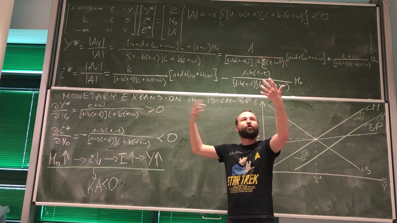
Monetary & Fiscal Policy in Open Economy IS-LM-BP Model
@lazarskiopencourses4059
559 views•2021-04-11
5:07
Impact of Yuan in Indo-Russian Trade Amid Sanctions
@WION
261.9K views•2022-07-01
10:33
Behavioral Economics Explained: Rationality, Nudges, and Risk
@crashcourse
1.1M views•2016-03-12

113:18
The Age of Easy Money: Fed & Inflation | Full Documentary
@frontline
21.2M views•2023-03-15
Related Study Plans & Knowledge Roadmaps
Structured learning paths in Economics
economics
Sovereign Debt: Defaults, IMF & Restructuring
01Introduction to Sovereign Debt & Government Bonds
02Debt Sustainability & Credit Ratings
03Anatomy and History of Debt Crises
+ 2 more learning modules
12h5 modules
Explore Roadmap
economics
Market Design: Matching Theory & Gale-Shapley
01Introduction to Market Design and Price-Free Markets
02Two-Sided Matching & The Gale-Shapley Algorithm
03School Choice Systems and Mechanism Design
+ 2 more learning modules
10h5 modules
Explore Roadmap
economics
Impossible Trinity: Forex, Capital & Policy
01Introduction to Monetary Policy and Central Banking
02Exchange Rates and International Capital Flows
03The Mundell-Fleming Model
+ 2 more learning modules
8h5 modules
Explore Roadmap
economics
Healthcare Economics: Market Failures & Systems
01Introduction to Healthcare Markets and Market Failure
02Asymmetric Information and Adverse Selection
03Moral Hazard and Insurance Design
+ 2 more learning modules
12h5 modules
Explore Roadmap