JPEG Compression Explained: Signal Processing & DCT Math

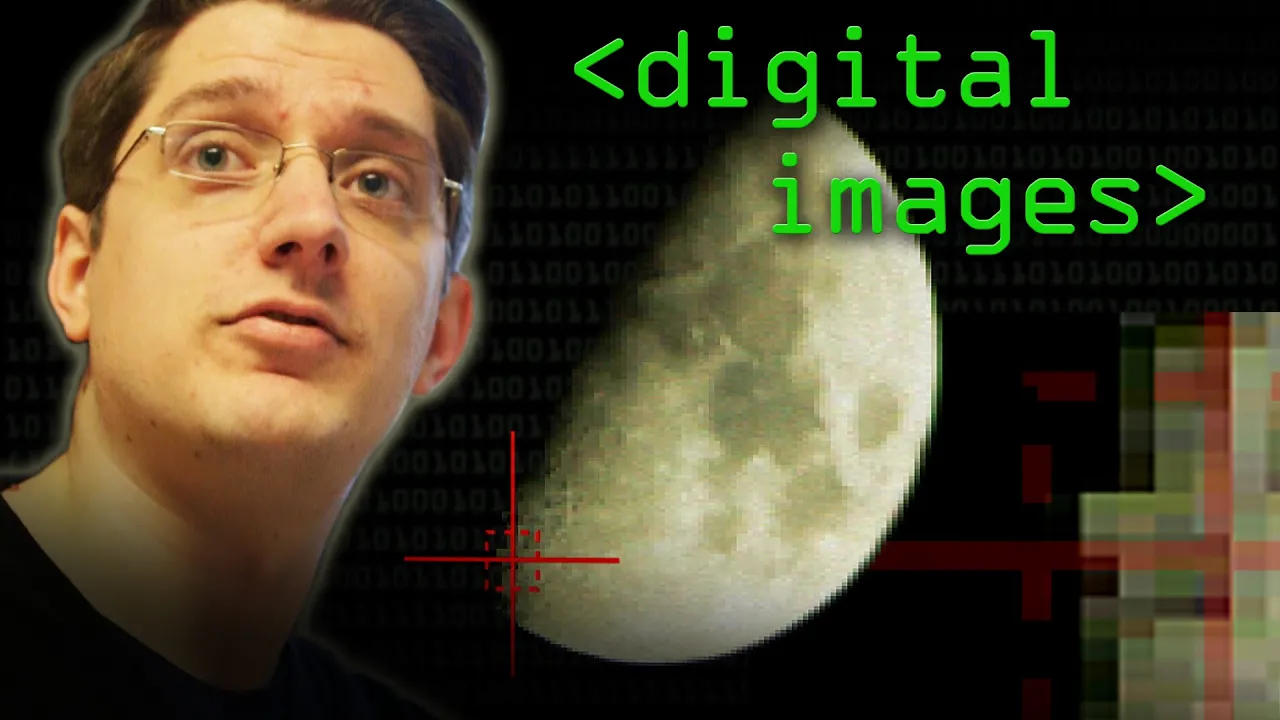
[00:00:00]what you see here is one part of a really elaborate process that defines the universally used jpeg image compression format jpeg is rather complex and in this video the majority of the focus will be on understanding how computer scientists came up with an algorithmic and mathematical framework for solving the complex problems that image compression presents but to understand the motivation behind the ideas in jpeg we'll have to dive into the inner workings of the many components involved the perspectives we'll take will be a little bit unorthodox but my hope is that you come away with a better understanding of the big themes in image compression which apply to other compression related problems it's not an exaggeration to say that these concepts are used every time you open an image play a video or listen to some music as we go through jpeg we'll interact with the wide variety of beautiful ideas in the world of data compression and signal processing that make the technology around us possible before we dive into jpeg let's talk about how computers represent images the standard color space that computers use is the rgb model every pixel of an image stores three values from 0 to 255 with higher values representing a larger weighting of the respective color so assuming each color component is expressed in 8 bits or a single byte of memory an image has 3 bytes per pixel here's an image with a little more than 5 million pixels based on our assumptions the total size of this image should be about 15 megabytes but with jpeg compression the actual file is only 0.8 megabytes same number of pixels but 5 of the expected size and the image looks absolutely beautiful this is the real magic of jpeg compression jpeg aggressively takes advantage of several clever ideas to achieve seemingly ridiculous amounts of compression with minimal effects on the quality of the original image one of the primary reasons jpeg works so well is it uses lossy compression to understand what that means let's think about compression from a big picture perspective we start with an rgb representation of an image and then we encode it using a compression algorithm this is what we store in memory and it's more compact but quite different than our original rgb representation so part of a compression scheme requires also defining a decoding component that converts the stored representation of our data into the rgb format that a computer can render as an image part of the jpeg standard is defining how both the encoding and decoding work a key point in jpeg is that the final decoded image is not going to be the same as the original uncompressed image that's why we call it lossy compression in the compression part of the pipeline we are going to deliberately lose information to get compression on the levels of five percent there's really no other option other than to actually discard some information from our original image now the fun question to ask is what sort of information from an image can we get rid of and how do we get rid of it answering this question is going to be the primary focus of our journey into understanding jpeg here's an interesting image for you if i were to ask you what colors the squares of a and b were i imagine most of you would quickly say that a is a darker shade of gray than b but what if i told you that a and b were actually the same color it's okay if you don't see that this picture is designed to trick our visual system but once we have a connector of the common color between the two squares it's much easier for us to see that they are in fact the same color so what's going on here over the years scientists have developed a human visual system model through the study of our eyes and one incredibly interesting finding through experimentation is that our eyes are much more sensitive to brightness than they are to colors and part of the jpeg compression scheme can take advantage of this but to understand how we have to dive into the world of color spaces as we've discussed the rgb color space is a combination of red green and blue color components if we put each value on a separate axis in a three-dimensional space we can see how all the possible colors are just a point on this cube one aspect of rgb color space is as you progress on the diagonal from the origin to the color 255 255 255 you get gradually brighter colors and in fact the exact line between these points defines all possible grayscale colors which are a direct measure for brightness this idea of separating brightness is core to another color space called ycbcr ycbcr stands for y chroma blue and chroma red our y component is going to measure the luma or brightness of an image and our cb and cr components are going to encode the colors if we look at the color space the y can be thought of as a single vertical axis with larger values encoding more brightness every cross section of the space defines a range of colors at that particular brightness for our purposes with jpeg using the color space gives us direct access to the part of color that our eyes perceive best as a result of being more sensitive to brightness than colors one idea to compress our original image involves sampling less of the cbcr components and keeping all of the luma components the technique is referred to as chroma down sampling or more commonly chroma subsampling suppose i have this 8x8 image which has the following y cb and cr components the key idea of chroma down sampling or subsampling is to take fewer samples from cb and see our components since our eyes are less sensitive to them here's one approach that defines a 4-2-0 chroma down sampling scheme we go through our original 8x8 image in 2x2 blocks and simply average the group of pixels to get a shared value of the 4 pixels in the original image averaging the pixels by the way is all downsampling really means chroma subsampling is the same exact idea but instead of averaging we just choose one of the samples usually the top left pixel to be the color of the entire 2x2 block once we have these fewer samples from the color components we can merge them with the luma component which will retain the original 16 pixels and this gives us our sub sampled image in this case you can see quite a difference since our 8 by 8 pixel image is significantly scaled up but in real world images it's often hard to see any changes after sub sampling by merging 2x2 blocks on the cb and cr channels into one color we are left with a quarter of the original data in each color channel shrinking the total file size by fifty percent we're still quite far from the five percent levels that we saw in jpeg so we're going to have to exploit more than just human perception of brightness for the following components of jpeg let's focus on the y channel which essentially defines grayscale images the principles we'll discuss from here on out will also apply to the color components of an image the next clever idea in jpeg requires looking at images in a completely different perspective one that can be a little bit counter-intuitive one way to think about images is treating them as signals if i slice a particular row of an image i essentially have a row of pixels each with some value between 0 and 255.

[00:08:32]if we plot these values we can get an approximation of a signal visualizing an image as a signal allows us to talk about frequency components within an image higher frequency components correspond to rapid changes between pixels while lower frequency components are related to smoother changes between pixels there are two key aspects of frequencies within images that are incredibly important to jpeg compression the first is that a lot of real world images shot from cameras are mostly composed of lower frequency components in other words if i take a random portion of a realistic image it's pretty likely that the pixels in that area do not change that rapidly and the second key fact is that from a variety of experiments the human visual system is generally less sensitive to higher frequency detail in images jpeg takes advantage of these ideas by strategically removing less important and less common higher frequency components from an image to achieve even more compression but there's one big problem how do we get frequency components from an image this is where some particularly clever and beautiful math comes into play the answer to this question lies in a special operation called the discrete cosine transform or the dct the dct works for any size input but to simplify things let's focus on an input of 8 pixels just as we did earlier let's suppose these 8 pixels form some sort of signal we'll never be sure what exactly the signal looks like since we only have 8 points but the clever and definitely not obvious idea of the dct is to represent these eight points as sums of sample points from cosine waves and i really want to emphasize the fact that we only care about the discrete samples visually i think it's nice to see the continuous signals and cosine waves but throughout our discussion the only values that really matter are the sampled points from these functions the dct takes an input of sampled points from our original signal and gives us an output of the same size we'll refer to the outputs of the dct as coefficients these coefficients represent the weights of cosine waves of different frequencies that contribute to the original signal a nice analogy is to think of this as unraveling a complex signal into a weighted sum of simpler cosine waves if you've never interacted with this type of idea before it's natural to be confused what cosine waves do we even use how do cosine waves relate to pixels on an image none of it makes any sense don't worry these are important questions that we will answer let's start simple and talk about cosine waves here's a graph of cosine from 0 to pi i've given you this general notion that the dct is supposed to tell us how much of a specific cosine wave is contained in a signal so let's test this out what happens if i provide an actual cosine wave as the input signal to the dct what do we expect to happen okay we can try this but there's a problem to follow our existing example we need eight sampled points from the cosine wave to make this work how exactly should we sample the cosine wave well there are a few options but let me present to you the most common one what we can do is split out cosine wave's domain into 8 even slices and then we take the midpoint of each of these slices this gives us the following input points which we can generalize for any number of points but for our purposes we'll stick with the smaller n equals 8 example so going back to our question what should we expect the output to be when we pass in sample points from a standard cosine function this is an interesting experiment when we pass these points from a cosine wave into a dct transform we get the following output only one coefficient has a non-zero value meaning there's only one cosine wave that contributes to our input and that seems to make some sense since the input is literally from a cosine wave in this case the first index is the only coefficient with a non-zero value when trying to understand complex ideas it really helps to play around with these simple examples a cool follow-up to our experiment is to see what happens when we change the amplitude of this cosine wave the first index dct coefficient increases if we flip the cosine wave by multiplying negative 1 the dct coefficient changes sign it's exactly acting like a weight for a cosine wave when the amplitude of the input cosine wave changes the weight correspondingly reflects that change so taking a step back how does this relate to images well just as we took images and represented them as signals the reverse also works standard grayscale images have pixels ranging from 0 to 255.

[00:14:16]the intuition with cosine waves to images makes more sense when we shift the range of pixel values by 128.

[00:14:24]with pixel values from negative 128 to 127 we can see a better mapping between this cosine wave to an actual set of 8 pixels this particular wave is a nice way to represent a row of gradually decreasing pixel values and the magnitude of that change as well as the direction of the change is reflected in the amplitude of the original cosine wave and consequently the dct coefficient so let's continue this experiment to see what else we can uncover about the dct we've messed with the amplitude of a cosine wave what other parameters could we change a simple one is to just shift the cosine wave up or down let's see what happens when we try that it looks like shifting up or down the signal only affects the zeroth index coefficient that's an interesting data point that we'll come back to another parameter of cosine waves is the frequency what we're going to do now is show the dct coefficients as we wind up the frequency of this cosine wave i'll keep the sampling strategy we discussed earlier consistent among all frequencies let's see what happens as we increase the frequencies we get a few different dct coefficients for the respective cosine wave that is until we get to this cosine wave for this particular cosine wave only the second index has a non-zero coefficient this cosine wave is actually just double the frequency of the previous cosine wave this is super interesting the first index of the output seems to nicely correspond with the cosine wave of frequency 1 while the second index correlates with a cosine wave of frequency 2.

[00:16:17]let's continue this experiment of increasing frequencies but before i continue see if you can take a guess at what frequencies the other coefficients will correspond to here we go we slowly increase the frequency and boom the index 3 coefficient corresponds to a cosine wave of frequency 3.

[00:16:37]then frequency 4 comes next and this pattern continues until we get to a cosine wave of frequency 7.

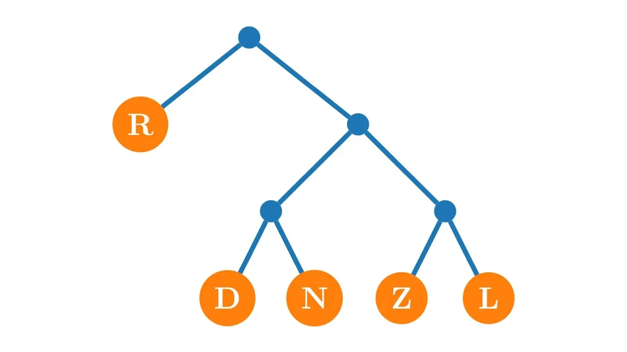
[00:16:45]pretty insane right so for the coefficients indexed one to seven it looks like they represent the weight on a cosine wave with the frequency that matches the index so what about the remaining index zero we saw shifting cosine waves up and down led to a change in the zeroth index what cosine wave does that represent some of you have probably figured it out but if you think about what a zero frequency cosine wave is it's just a constant signal what that means in terms of images is it gives us a measure of the overall brightness of a set of pixels brighter images will have a larger zero to coefficient than darker images this is why shifting up a cosine wave only impacts the zeroth coefficient putting this all together each of these frequencies correspond to a different pattern of images and what the core dct does is break down how each of these fundamental patterns contribute to the original image and it turns out that all possible combinations of 8 pixel values can be represented as a sum of these eight cosine waves why that's true is not at all obvious but we can begin to understand it once we translate this intuition to the actual math behind the dct if you look at the mathematical definition of the dct we usually have a vector definition of the original signal and the output coefficients we want to define the kth index of the coefficient vector mathematically what you often see is something that looks like the following and with the intuition that we just built up we'll see that this equation is doing exactly what we want let's start with the cosine term this function should be familiar it's the exact representation of a sampled point from a cosine wave using our earlier sampling scheme and it incorporates the frequency of the cosine wave as well now what's interesting is in order to get the kth index we are actually summing over a product of each sampled point with samples from the cosine wave why does that make sense this type of expression might look vaguely familiar to a lot of you let me rewrite this another way we know that the original signal points can be represented as a vector but what if we rewrote the sampled points from the cosine wave as a vector as well what does this expression mean in the context of these two vectors it's a dot product and what we know about dot products is they're a nice way to measure similarity between two vectors that's why when we pass in sample points from a cosine wave of frequency k as the input to the dct we got large values at the kth index coefficient these two vectors were just scaled versions of each other so the dot product was maximized and this perspective reveals what i think is truly the most surprising and elegant part of the dct by picking the points through the sampling method we can think of the entire dct as a matrix vector product all we're doing here is a linear transformation the rows of the matrix are the sampled points from the cosine waves of the respective frequencies and what's truly astounding is that all row vectors in this matrix are orthogonal to each other what i mean by that is if you take the dot product of any two row vectors representing cosine waves you will get zero if they are different rows of the matrix intuitively this is why in our earlier experiments when we pass in a cosine wave of a particular frequency as an input into the dct we didn't get a contribution from any of the other coefficients which represented different frequency cosine waves the orthogonality of the sampled points from different cosine waves generates this behavior it's really quite beautiful another great property of the dct that follows from these facts is invertibility i've talked about the dct as a way of decomposing a signal into a coefficient representation of weights associated with cosine waves we can also reverse this process if i take my coefficient representation of the signal i can apply what's called the inverse dct to get back the original signal and it is the exact same signal no information is lost in this step how we do that is by multiplying our coefficient representation with the inverse of the matrix what's cool about this is that because of the orthogonality of the vectors the inverse is just the transpose of our original matrix with some additional normalization constants now there's a super nice interpretation of the inverse dct the sample cosine wave points are now column vectors so what the inverse dct is doing is essentially summing over a weighted combination of cosine waves directly to get the original signal and because these columns are orthogonal to each other that's what allows us to represent any set of eight points with these eight cosine waves absolutely incredible i know we spent some time and went through some fairly complex math to get here but it's precisely these details that are the most fundamental part of not only the dct but many other similar transforms in the world of signal processing now that we have a good intuition on the one-dimensional dct let's talk about how jpeg specifically uses it jpeg takes an image and splits it into 8x8 blocks and then centers their values around 0 by subtracting 128 then we take the block and apply the dct to each row of the block giving us eight sets of dct coefficients we then apply the dct to each column of the block this process is what defines the two-dimensional dct so in the end we have 64 coefficients each of which are a weight on a specific 8x8 pattern notice the first row and column correspond to the earlier one-dimensional patterns and the other elements are compositions of these patterns and just like in the one-dimensional case the big idea here is that we can build up any 8x8 image using these 64 fundamental patterns the same signal perspective we talked about earlier also applies here except now with 2d waveforms what's going on here is we are plotting the pixel value on the z-axis with brighter pixels having larger values what's fun to play around with is seeing how the waveform and image come together as we slowly put together the 64 coefficients in increasing frequencies seeing this in action makes you realize that one interesting property is that by the time we incorporate a small portion of the coefficients our signal and image already look pretty close to the original versions there's an even more direct experiment we can run to quantify this notion this particular 8x8 block was randomly picked out of the original image if we map out the magnitude of the dct coefficients on this block we see that most of the largest values are in the upper left section which corresponds to lower frequency components and what's even more interesting if i take any 8x8 block on this image almost all of them have the same property this property of the dct is what's commonly referred to as energy compaction after applying the dct most of the largest values are concentrated in a few low frequency coefficients and this holds true in a lot of real world images the concept of energy compaction is incredibly important in image compression as we will see it's exactly the property that will allow us to aggressively compress images while still retaining high visual quality fun fact the original discovery of the dct centered around approximating other transforms that had better energy compaction properties but were too expensive to carry out the dct is just one example of a transform that has this property for real world images and we use it because it's quite easy to compute there's a lot of complexity involved here but one of my goals in this discussion of the dct and jpeg was directly interacting with these deep and important ideas through questions and visual experiments interactivity is a core part of learning and a website that does a fantastic job of interactive explanations is brilliant the sponsor for this video from the basics of mathematics and algorithmic thinking to more complex ideas and deep learning and probability brilliant offers a variety of courses and learning paths for those interested in getting hands-on practice our discussions of jpeg interacted with some linear algebra in the application of image compression and brilliant has an entire linear algebra module that goes through the fundamentals and even shows applications of these ideas in image compression cryptography error correcting codes and much more when i was a student i really enjoyed their computer science fundamentals course which has engaging visualizations of concepts and great practice problems that helped me solidify my foundations you can get started for free by going to brilliant.org reducible which is linked in the description below brilliant is providing a special offer through this channel where the first 200 members to sign up get 20 off the annual subscription it's a great way to learn more about the topics in these videos and also a good way to support this channel big thanks to brilliant for sponsoring this video let's put everything we've discussed with the dct together in one more experiment we'll split our image into 8x8 blocks and then basically rebuild the image with each block having only a certain number of dct coefficients we're going to start off with zero coefficients and slowly build up the image after one coefficient we end up with basically a blur of the original image and as we add dct coefficients slowly notice how quickly the image starts looking like the original by the time we get to less than 25 percent of the dct coefficients you almost can't even tell the difference between the two images this confirms the key aspects of why jpeg works for this particular image almost all the blocks are composed of the lowest frequency components and we are generally less sensitive to changes in high frequency details so at this point we know we can eliminate higher frequency components from the dct but the next natural question is how we actually do this the process for eliminating higher frequency components in jpeg is called quantization quantization is a simple idea given an 8x8 matrix of frequency coefficients from the dct what we're going to do is basically divide each element by a scalar value and round it to an integer these values are defined in terms of a quantization table notice larger values in the bottom right of the table leading to zero values in the higher frequency components in the decoding stage of jpeg we'll actually be multiplying this result by the same quantization matrix element by element and as you can see the final coefficient matrix will be quite different from the original one so what that means is we're purposely losing information in this step but the key idea here is most of the lower frequency components will be retained this is why the energy compaction property of the dct is so useful when the largest values lie in the lowest frequencies we will end up with a lot of zeros in the less important high frequency components these quantization tables are provided by the jpeg standard from visual experiments and are the main way for jpeg to define quality of compression high quality compression parameters can be translated to lower quantization table values in practice jpeg also defines a separate quantization table for both the luma and color channels notice that in the color channels quantization can be even more aggressive after performing quantization we have a matrix of quantized dct coefficients where we can now exploit redundancy to get even more compression the last part of jpeg encoding involves a combination of run length encoding and huffman encoding one clever trick is that a jpeg encoder will order the coefficients in a zigzag manner to maximize the chance of a large sequence of zeros in order classic run length encoding can compress this fairly easily all that's going on here is we are compressing every sequence of zeros into a count of the occurrences in a continuous sequence jpeg actually performs something a little bit more sophisticated by keeping track of a triplet for every coefficient this triplet encodes the number of preceding zeros the number of bits required to encode the coefficient and finally the actual coefficient value we also have an end of block value to signal that everything from here on out will be zeros [Music] this particular scheme works well with huffman coding to further exploit redundancy the big idea of huffman codes is that more frequently used data can be encoded with fewer bits and it turns out especially with the nature of quantization these triplets can be further compressed since some of these values will be more frequent than others however i'm purposefully not going to go into the details of how jpeg uses huffman codes to compress the data because it really does get quite tricky to give you some sense of the problems we have to deal with encoding signs of coefficients as well as triplets for all 8x8 blocks most encoders also encode the top left coefficient separate from all the other coefficients and when you handle that you have to deal with this on both luma and color channels and when you eventually get that working a good chunk of your logic will break when you have to deal with the different types of chroma subsampling implementing an optimized fully functional jpeg encoder and decoder is no joke i wouldn't give that task to even my worst enemies but in terms of the big picture all that's going on in this component is taking advantage of the redundancy that quantization creates a jpeg decoder will be able to use the huffman code data in the files to get back all quantized dcd coefficients that were encoded this part of the jpeg algorithm does not lose any information jpeg as a whole brings about an interesting discussion on the philosophy of data compression the classic and most straightforward way to compress data is by taking advantage of redundancy this is the basis of losses image compression algorithms such as those found in png file formats in fact for images where it's really important not to lose any information png format is recommended over jpeg but on most real world images being aware of the medium of presentation introduces another really powerful perspective a lot of innovation in jpeg compression comes from experiments and understanding of human visual systems it's from these experiments that we realized human eyes are less sensitive to color and also less sensitive to higher frequencies so we can remove that information without a significant visual impact this is why jpeg is so much more effective at compressing images than lossless formats you'll find these same types of techniques used in audio and video compression where algorithms use our perceptions of sound and motion respectively to remove less relevant data in fact variations of the discrete cosine transform and quantization show up in both audio and video compression it really is incredible to me how people in these fields came up with the mathematical and algorithmic framework to utilize the way we actually perceive the digital technology around us there's so much depth to these topics that i could never hope to cover in just one video but i do hope this gives you a sense and appreciation for the complexity of the technology around us that we use on a daily basis thanks for watching and i'll see you all in the next one