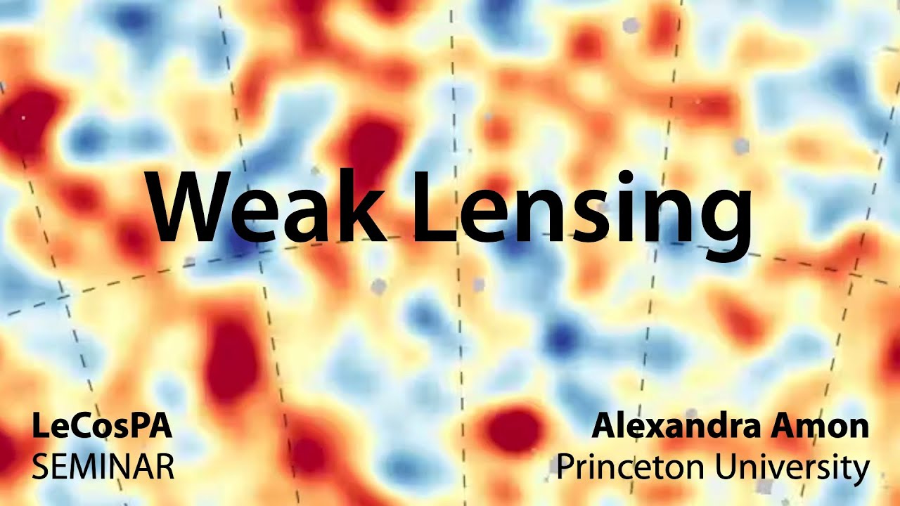
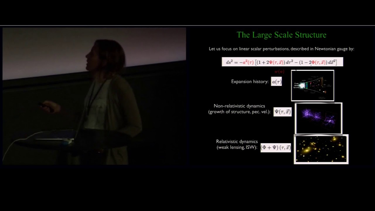
Weak Gravitational Lensing: A Comprehensive Guide | ISSSA & RCAA 2022

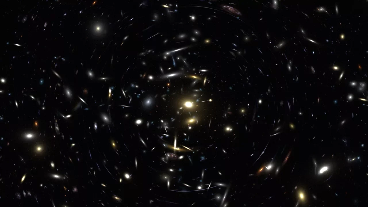
[00:00:00]okay um hello everyone i'm sure moray and it's a pleasure to be back again here to convey uh this particular set of lectures on gravitational lensing um i started off with this series of lectures with an introduction to gravitational lensing um and the basic equations uh which govern gravitational lensing then yesterday you heard from anubrita who told you a little bit more about strong gravitational lensing and how the equations that we have derived previously um how they can be used um in order to uh in order to learn about the matter distribution in galaxies especially when there are multiple images forming and you can you can study the properties of these multiple images such as the locations where they are formed uh then their individual magnifications um as well as the time delays coming from these images right so we have derived a formulae in the first set of like in the first lecture in the second lecture you saw how they can be used in order to learn a lot more about the universe in this third lecture i'm going to talk to you about weak gravitational lensing so this is a slightly different form of gravitational lensing nevertheless uh but it's less majestic than the strong gravitational lenses that you're used to um and so but nevertheless very useful and very powerful so let me introduce that to you so before we begin again let me show you this picture of gravitational lensing happening within a galaxy cluster so you can see these foreground galaxies these elliptical galaxies which are in the foreground and then the background galaxies which are getting lines so you can see these arcs sometimes there are these radial arcs that you also form here as well here right sometimes you see these merging images where two images which are of the same object are forming very close to each other and even here you can see this image and this image it's a pair of merging images okay so this is all beautiful right lots and lots of stretching and multiple images being formed but the the topic today will be of galaxies which are just weakly distorted okay so these galaxies are very well aligned with along the line of sight to this cluster and that's why they get these multiple images but if you're not very well aligned if your beta is very far away from the object that is causing the lensing then you don't form multiple images instead you form just a single image but it's a little bit distorted not as [Music] the distortion is not so large that it causes arcs but nevertheless you see some tiny distortions some changes to the shapes of these galaxies and it is these changes that we are going to try to focus on so what is weak gravitational lens okay so i'm showing you this cartoon picture of what we gravitational lensing does and then we will get to the equations behind okay so what you are seeing here are pictures of galaxies which you can see on in the observed sky right so these galaxies are actually located in the distant universe like here right and this is the picture that you see eventually on the sky right that's the projected picture that you see now each of these galaxies this let's consider this blue galaxy which is here so that particular galaxy [Music] there are bundles of light rays right which are coming from these galaxies coming from different portions of these galaxies so these bundles of light rays they travel towards us and then they encounter some matter distribution in between right like these vests ghost like structures that you see here which are the dark matter distribution which is supposed to represent the dark matter distribution so it encounters this dark matter distribution and then these bundles of light rays each of them gets deflected by a slightly different amount right and so when these deflected light rays eventually come towards you and you see them in the sky then what happens is that the bundle of light rays that started off it doesn't remain the same bundle it gets a little bit distorted right and so the shape of this galaxy which you see here originally it should have looked like this in the absence of dark matter when there is lensing which is happening after that the shape of that galaxy has changed it has rotated it has stretched a little bit and so on right similar thing happens for this galaxy this galaxy these galaxies so all these background galaxy they get distorted the shapes change as they come towards us right and this lensing this distortion in these shapes it's happening because of the presence of this start now lensing is also sensitive most sensitive to the structure which is roughly halfway in between us and um and the source okay so these galaxies when they will get lengths they will be most likely due to lenses which are some roughly halfway in between that is where lensing is most efficient and so what it means is if you look at the shapes of galaxies as a function of different distances away from us then they will be sensitive to the matter which is roughly halfway in between them and us but closer and closer to us or further and further away from us depending upon where these source galaxies are right depending upon the shapes of the galaxies that you are considering so if you have some way of identifying roughly what is the distance of any of these galaxies that you observe in the sky and you look at their shapes then you can do a tomographic reconstruction of the matter which is in between us and them so for example if you look at the shapes of galaxies which are really far away they tell you the distribution of matter here instead if you look at galaxies which are here and measure their shapes then that tells us about the distribution which is a little bit halfway in between uh those galaxies and us right so by doing this kind of analysis with galaxies at different distances you can do a tomographic reconstruction of the dark matter so this is what lensing allows us so to look at how to actually do these things let's look at the important equations that we have already studied uh you heard about a few of them yesterday and then i had covered them uh day before right so the first of all everything that you need to know about lensing you can derive from this quantity called the lensing potential right given by psi so this is related mainly to the surface density right this kappa of theta is called a convergence and this convergence is just the surface density divided by the critical surface density the surface density tells you about the mass distribution in the lens plane and the critical surface density it is a function of the the distance to the lens the distance from the lens to the source and the distance to the source itself right so it's a geometric factor that gives rise to this quantity called the surface density in addition to constant like c square and g right so you combine these distances and the fundamental constants you get out of surface density that surface density is called a critical surface density so kappa is just sigma divided by sigma critical and that is how you using this particular equation you can define something called the lensing potential the deflection angle is just the gradient of this lensing potential right this is again something which we are derived um we have worked out from first principles what the deflection angle looks like and then from from general relativity right and then from there we worked out what is the definition of a potential which will give you um the deflection angle when you take a gradient of it so these are the two equations and then there is a relationship between this lensing potential and the kappa itself right which is causing this lensing potential that relation is given by the laplacian of phi is equal to 2 times kappa so this is a poisson like equation so you can see the uh the similarity between these equations and the equations that you're familiar with right in the so there is a gravitational potential right you take the gradient of the gravitational potential you get a force right and then if you take the laplacian of the potential then you get back the density itself right so there is a commonality and similarity between these equations right so one is a 3d equation this is just an equation in 2d that's the reason why there is a log here instead of a 1 over r that you are used to okay good so then once you have this deflection angle alpha then it allows you to figure out if there is a source which is at a position beta then where will its image be right so if you know also if you know the deflection angle then given a source position you can figure out where is the image position so that particular equation is just geometry and i showed you that it looks something like this beta which is the original position is theta which is the position where the images image forms minus alpha of theta which is what is the exact deflection that happens at that particular uh image position right so beta is theta minus alpha of theta this is just represents the geometry of the lensing configuration and once you know the alpha value then you can add a beta value a given force position you can figure out where the image position should be okay then the next thing that we had also looked at is the definition of this of a quantity called the shear which tells you how bundles of light rays coming from a source how they get distorted right so we had worked out using this lens equation we had taken something called the jacobian of this equation by doing a differential so del beta by del theta because this is a vector equation there where there are two components to this vector in the plane of the sky and that's why for the jacobian you get four components so del beta by del theta has four components that gives you a matrix right and that matrix looks something like this 1 minus kappa minus gamma 1 minus gamma 2 minus gamma 2 here and then 1 minus kappa plus gamma and i told you what this jacobian matrix look does so you can split this jacobian matrix into these two components there's a one minus kappa times an identity matrix which is just telling you that you take a source it will just get magnified isotropically by a factor one minus kappa and in addition to that there is this component now this you cannot write it down as some number times an identity matrix so each of these axis are being scaled in different manner and that's why these components look different and so this shear component it tells you something about how a circular source get marked into an elliptical source so let's try to understand that a little bit more so this quantity gamma as we said it has two components gamma 1 and gamma 2. so it becomes easy to express it as a complex number okay there is nothing complex about it the only reason why we are expressing it as a complex number is because there are two components to it and we want to keep track of both these components so this gamma can be written as gamma 1 plus i gamma 2 and if you go from the source plane and if you had a circle with a radius r then when you convert it into an image in the image plane so as you will see it then it uh it turns out to be an elliptical just like the one you are seeing here and the major axis of this ellipse is given by the semi-major axis and the semi-minor axis of these ellipses are given by these quantities okay so r divided by 1 minus kappa plus mod gamma and r divided by 1 minus kappa minus mod so this is the major axis this is the minor axis right so so that's how these things get stretched and this mod gamma is nothing but the the modulus of uh the complex number that we defined before right so it is gamma is gamma 1 plus i gamma 2 and so mod gamma is square root of gamma 1 square plus gamma 2 so now we know if you know the magnitude of the shear what are the axis ratios that you will have right so if you have a source which is circular it will get mapped into an ellipse and the ellipsis axis ratios they will depend upon this value of mod gum right so if you look at it you can you can take this quantity and you can write it down as r divided by 1 minus kappa i can take it out times 1 plus mod gamma and then for this one it becomes 1 minus kappa 1 minus mod g sorry and this mod g is then defined as mod gamma divided by one minus star in most cases for weak lensing that we will be considering kappa will be much smaller than unity and so for all practical purposes for weak cleansing this mod gamma will be exactly equal to this much because kappa is small so in that case you take the axis ratio so you can take the axis ratios by dividing one by the other right and you will see that it is equal to one plus mod g divided by 1 minus mod g and so you can rearrange this axis ratio equation to get what is an expression for mod g so the modulus of the of of of the shear itself right is given um by the ratios of these uh ellipticity components right so or sorry the um the axis ratios b by a modified in these particular so if you know mod gamma then or if you know the axis ratio then you can figure out what is mod right so if you had a circular source you it becomes elliptical because of lensing you measure the semi-major semi-minor axis you define what is this b over a and you compute a quantity which looks like this it will tell you how much here it should have undergone right in order to become elliptical so this way you can map out the shear at different locations in this car so you take galaxies at different positions you measure their shapes when you measure their shapes they tell you about the shear itself which is present on this car okay once you know the shear then you know the lensing potential good so then we can also figure out so i told you about what is this mod gamma now let's try to understand what is the direction in which these galaxies gets stretched and in order to do this you just have to do a simple eigen analysis right so eigenvector analysis so let's suppose that eigenvector is oriented along the direction 1 and tan phi the eigenvector of this particular matrix right so the eigenvector of this matrix it will tell you in which directions you see the semi-major and the semi-minor axis okay and so to in order to do that eigen analysis what we can do is you can take the matrix you multiply it by a vector so let's suppose the eigen vector is in the direction someone tan phi right so that gives you uh so let's suppose that eigenvector has an angle which is uh phi with respect to the x-axis then the vector along that line is one time one comma tan phi and so you take the matrix you multiply by 1 comma tan phi and it should give you back the eigenvector times sorry the eigenvalue times the eigen so you can compute what the eigenvectors are one of the eigenvectors will look like this the other eigen vector will be 1 minus kappa minus mod and so let us consider this particular eigen vector and ask what is the relation of phi with gamma 1 and gamma so you take this equation and you just write it down so this is 1 minus kappa minus gamma 1 minus gamma 2 tan phi is equal to 1 minus kappa plus gamma times 1 right so so that's all the equation that i have written down the second equation is something which gives you exactly the same quantity so we'll just look at the first one and so you can rearrange this to figure out what is tan phi and tan phi comes out to be this and using the identity for tan 2 phi compared to tan phi which is given by this you are you can show that tan 2 5 is given by gamma 2 divided by gamma so the phase of this complex number right it should be uh 2 phi right so you can write down gamma as mod gamma times e to the i to sum right and that e to the i to phi is just cos 2 5 plus i sine 2 phi right and so if you take the ratio of gamma 2 by gamma 1 you should get tan 2 so this tells you that the ratios of gamma 2 by gamma 1 it can give you tan 2 phi where phi is the angle made by the major axis of the source with respect to the x-axis so this defines what exactly is the distortion that gets imprinted on a source which is circle right it becomes an ellipse and if you know gamma 1 gamma 2 then you can figure out what is tan 2 phi and then figure out the angle at which you will get the major axis that will be you take a tan inverse of gamma 2 by gamma 1 and then divide by 2 so this tells you how you can map out gamma 1 gamma 2 the whole shear field which is not a scalar right at every point there is a direction to this field and an amplitude to this field and so you can figure both of these things out by looking at the ellipticities of these objects so let me show you some give you some flavor of numbers right so because it's it's a little bit non-trivial because it has this 2 phi kind of relation so it's not easily it's not a vector and so it is not easy to visualize sometimes especially the first time you are hearing it so let me show you what a galaxy looks like if it has a gamma one which is greater than zero and gamma two which is equal to zero in that case that galaxy will be oriented like this the major axis will be along the x axis and the minor axis is along the y axis if instead gamma 1 is negative and gamma 2 is 0 then it means that the galaxy is oriented in a vertical now you can consider the other question which is what happens if gamma 1 is 0 and gamma 2 is greater than 0 or gamma 2 is less than 0. in that case the galaxy is oriented at 45 degree angle because of this two phi okay because tan will become infinity right and that's when uh 2 phi is equal to pi by 2 and so phi should be pi by 4 in that case so you see gamma 2 greater than 0 and gamma 1 equal to 0 means that it should be oriented at 45 degrees while gamma 2 less than 0 and gamma 1 equal to 0 it should be oriented minus 45 minutes so this is shown here what what are the different components gamma 1 gamma 2 and you can study these kind of figures in order to understand how these different gamma 1s and gamma 2s what are the different orientations of the ellipses that will in these different cases now let's try to understand what is the kind of ellipticity pattern that you imprint on galaxies that masses imprint on galaxies so in order to look for those kind of patterns first we have to understand what they look like right so let's consider some source galaxy population which is completely circular okay this is for simplicity now so this is shown here on the left hand side with these green dots all of them are perfect circles now let's put a lens in front of it so when you put a lens in front of it then the shapes of each of these galaxies it changes and you can see that the pattern it prints it looks something like this the thing that jumps out the the first thing that jumps out is if you are closer to the center the distortions that you get are larger right this we knew this was obvious nearer to the cluster center you used to get big arms so you can see as you are closer to the cluster center you get this larger distortions and as you move further away the distortions are smaller this is the first thing to remember the second thing is the pattern of the ellipticity is that getting printed so if you have a circular axially symmetric mass then it introduces a tangential ellipticity pattern so all the shapes get oriented tangentially with respect to the mass that is kept at the center of this distribution of galaxies so these kind of patterns if you look for them if you see this kind of pattern suddenly in the shapes of galaxies in the sky then you know that there should be some mass here which is causing these patterns the problem behind all of this is that background galaxies are not inherently circular right so if you look at intrinsic galaxy shapes you know that they are not certain right there are many spiral galaxies in the universe and depending upon the inclination angle of these spiral galaxies they will appear to be elliptic right not i mean the isoforce will appear to be ellipsis right and so this for example is a uh is a galaxy which is a job right while there may be galaxies which are face on and then they might look circular right so galaxies themselves they are not inherently certain so this causes a problem because now when you measure the shape of one galaxy you cannot infer really what is the shear at that location because that shear is contaminated by the intrinsic shape of the galaxy which is not circle so that's why what you have to do is you cannot use this method of measuring the shape and inferring the shear on a galaxy by galaxy basis instead you have to do it statistically so what do i mean by statistically you take many different galaxies say suppose in this particular patch right and you average out their ellipticities then what will happen is if you these galaxies are completely unless when you average out these ellipticities because galaxies on average will be completely randomly oriented and so when you average it out the average ellipticity intrinsically of these galaxies should be zero but when there is a mass which is causing the lensing and now you average the ellipsis of these galaxies here you will see that the average ellipticity will be aligned in this particular tangential map again with respect to the center of this mass distribution so you do it here you do it here you do it here you do it in different different locations and that will allow you to figure out this coherent pattern of ellipticities which gets introduced because of lens this happens because these galaxies are almost experiencing the same potential from these central object right and so that's why they are sheared coherently in a coherent path and that's the reason you can statistically average it out and then figure out what this shear is so by all this you must have understood now that the most important thing for weak lensing is then to measure the shapes of galaxies right and so the question is then how do you measure the shapes of galaxies right so we get these pretty pictures in fact the actual galaxies for whom we measure the shapes are even dirtier than what you're seeing looks right but let me show you um to begin with show you a galaxy where at least you can see the uh the galaxy properly right and it's well measured so the first thing to measure the shape is to figure out where is the centroid of this galaxy so in order to measure the centroid you can calculate it using moments of the surface brightness distribution so you take us the surface brightness distribution and you take the first moment of it so multiplied by theta integrate over the entire plane of the sky typically over a small region which contains the light from the galaxy and then you divide by the same factor right d2 theta i of t this q i is just some weight function which tries to downward the intensities which you would have measured with very low signal to noise ratio right so further out from the galaxy center you don't want to give too much weight because it's noisy right um and so that's all what this qi is done but otherwise it's just the first moment to measure where is the center of this house once you measure the center of this galaxy then with respect to this center you can measure the second moments of the surface brightness distribution so that is what is shown here you again do i of theta times q i this is the waiting function and then the second moment that you are measuring will be theta i minus theta i bar theta j minus theta j bar right so this second moment again will be uh uh we'll have four components right because you can do theta one minus theta one bar theta one minus theta one bar or theta one and then j might be two then i becomes 2 j becomes 1 i becomes 2 j because right so all these i j they're taking all sorts of indices 1 comma 2.

[00:28:09]and so you get a 2 by 2 matrix again for the second moment measurements so once you measure these second moments you can define the ellipticity in this particular fashion okay so what is this number so q11 minus q22 plus 2 times iq122 divided by this this kind of complicated denominator that you see but let's try to simplify and try to understand it let's suppose you have a galaxy which is completely gaussian and this gaussian is oriented along the x y axis let's suppose that that is the case in that case this term q 1 1 it will tell you what is the sigma square along the x direction while q 2 2 will tell you what is the sigma square along the y direction so this sigma square is giving you some information about the width of this object right and that's why this q 1 1 minus q 2 2 will be equal to a square and d square where a and b are the major and the minor axis and so these things are related the main moments are related to these um the size of these major axis and minor axis and then q one two will be exactly equal to 0 because you are integrating along one axis and then along the other axis so so that will give you 0 and now what you will do again is now let's consider the denominator which is again a square plus b square right and so you have a square minus b square divided by a square plus b square that gives you a minus b divided by a plus b sorry this is a square plus b square plus 2 times a times b right so this you can write it down as a plus b the whole square and so this a square minus b squared divided by a plus b the whole square that will give you a minus b divided by a plus b that quantity is just 1 minus the axis ratio divided by 1 plus axis 1 minus b by a divided by 1 plus beta and if you remember 1 minus b by a divided by 1 plus b by a this was related to the actual magnitude of the shield so if you can measure the shapes of these galaxies you can measure the magnitude of the shear by looking at the by looking at these second moments and defining an ellipticity which looks like this okay good now as i said galaxies are not circular even without lensing and so they have intrinsic elasticities but they are expected to be randomly oriented so if you average out many many galaxies then you can figure out what is the actual shear at the location of this galaxy so you can ask how is the intrinsic ellipticity of sources related to the observed electricity and the shear at the location of the galaxy so this involves some matrix algebra but it's it's again not too complicated and you can show that this actual intrinsic electricity of the source is related to the observed ellipticity of the source and the reduced shear with these particular equations and now if you average over intrinsic ellipticity we know that when you take that average you should get 0 and so you can now average the intrinsic ellipticities here and you can show that the average of these observed ellipticities then is equal to either g or 1 over g star depending upon whether your modulus of b shear is less than or equal to 1 or greater than this particular quantity is of less interest because this happens very close to the center of the cluster so we will not be considering this particular part but it's mainly this particular equation that gets used right so you take the ensemble average of the observed ellipticities of galaxies and it tells you what is the reduced shear at that location and if you are in the weak lensing regime the reduced shear is same as the shear at that particular machine okay okay so now that we have many many galaxies we have made measurements of the shapes of many of these galaxies we know where they are oriented then we can figure out what is the value of the shear and what is the orientation of this so we know exactly what the value of shear is at different positions on this tank right we have done an ensemble average of a few galaxies in a certain small region and then calculate what this value of shear is now how is that shear use right that shear is being caused by matter distribution in between so let's try to figure out how to infer that matter distribution from the observed in order to do that we have to start from the equations that we actually learned before in the first lecture right so one of the things was there is a relation between the lensing potential psi and the kappa value which is the poisson equation right so you had laplacian of psi is equal to 2 times kappa now you can take psi which is this lensing potential and you can decompose it in fourier space right and so the fourier expression will look something like this psi tilde of l is equal to integral of d theta e to the minus i l dot theta times r so you can do a fourier decomposition again in 2d right so that's why you have this minus l bar dot theta and once you start with this equation now you apply the laplacian on this right then um you you get a minus i l down and then you apply uh i mean you take the gradient then you get a minus il down you take the laplacian you get another minus il down and so in the end you get minus models on the on the left hand side minus model square times psi of r that's what the laplacian gives you and that is equal to 2 times kappa and so again you are taking it in fourier space and so that's why it becomes 2 times kappa of l this minus sign which was here i just took it here that's what so this is the fourier space equivalent of the poisson equation good so how does this help let's go through it again slowly so we also have the definition of what gamma 1 and gamma 2 is with respect to the lensing potential that definition was given by these two quantities it were these were derivatives in the lensing plane right so this is psi one one so you take along the x axis the derivative of the lensing potential two times delta two psi by del theta one square and then subtract delta psi by del theta two square and take half that is what is gamma 1 gamma 2 is just delta psi by del theta 1 delta t so this is the definition of what gamma 1 and gamma 2 looks like and the shear mod gamma that you can write it down as gamma 1 plus i gamma 2 so now that we have this fourier equation for [Music] we have we are doing things in fourier space so we'll express this i 1 1 also in fourier space so when you take this derivative with respect to theta 1 or along the first direction the x axis direction then you get a l 1 square and here if you do it then you get a l2 square so what you get in the end is l1 square minus l2 square divided by 2 that's exactly what you are seeing there is l1 square minus l2 square divided this comes from this component and then psi 1 2 which is related to gamma 2 you can imagine it gets l1 times l this i we have just put in by to just separate the components for the for the shear so now you have what gamma looks like in terms of the lensing potential but this lensing potential is related to kappa by this poisson equation so now you can take this model square down right and replace psi of l by kappa divided by model square so you now get an equation between shear and kappa but in fourier space and it looks something like this you can also take this quantity and move it to the other side and you can see that kappa of l is also given by 1 minus 1 divided by model square times again this kind of a kernel multiplied by gamma so if you know kappa of l you can predict what is gamma l if you know gamma of l then you can predict what is cup of so it's a simple relation between kappa and gamma which allows you to go from one to each other the relation is much easier in fourier space than it is in real cities and you can also see there are many similarities between the two right except for this plus i going to minus i there is no difference between these two equations when going from one to the other right kappa to gamma and gamma so this also helps us to write down what is finally the equation going to be for kappa so if you have measured gamma you can put it on a fourier you can calculate it as a in the fourier domain itself if you have computed the shear in the fourier domain you apply these equations you can get the conversions in the fourier domain this is just sigma divided by sigma grid and so if you know all the length source distances etc you can figure out what is the surface lenses so that's how you can go from measured values of shear to measured values of this quantity kappa which is related to the surface density now let's go one more step back to figure out what are the radiation what is the relation between the potential and kappa but in real space for that you should consider first the equation for the deflection angle which you get by taking the gradient of the potential that's why it's psi i so that is 1 over pi integral d theta prime kappa theta prime and this kind of deflection equation that you are used to uh if you are in a for a point mass you can see this that it looks like 1 over mod theta it's just in towards the direction of that point so this is the definition of psi then you can take another derivative so you can work out what is psi i j it will look something like this you can see this direct delta function coming because there is a theta i here right and so on so you can go through these equations and show that this is indeed the case and we have the definition of gamma based on these derivatives of the potential right and so you can use these equations gamma 1 and gamma 2 equal to this you can substitute i and j for 1 comma 2 into this equation and you can write down the relation between gamma and kappa in real space has this particular quantity so you see gamma is related to is is some sort of an a convolution integral of a corner with the surface density or with the convergence so this is a convolution operation okay because i have an integral over some variable i have a kernel which is theta minus theta prime right and then a surface density another field so convolutions are typically simpler in fourier space and that's why you just saw multiplications in fourier space when we saw these equations so that's why you can go from one to the other and in real space it should look like a convolution and that's exactly what you do now given that the relation in fourier space for gamma and kappa it looks fairly similar you can also expect the relation in real space to go between kappa and gamma to also look similar and that's exactly what happens so the only things that change this theta 2 square minus theta 1 square remains the same instead of minus 2 i theta 1 theta 2 we just have 2 times theta 1 theta 2 remember i have written this as a vector i could have easily written theta 2 square minus theta 1 square plus i 2 theta 1 kt this is the same thing so you can go from gamma to kappa by doing this convolution you can go from kappa to gamma doing this kind of convolution that's all so you can reconstruct what is the mass density in between us and the galaxies by by measuring the shear itself and using these equations so this is quite possible now there's another quantity which is very important you remember if there was a point pass at the center of an unless distribution then the galaxies they get oriented in the tangential so rather than figuring out all the shears at each and every location in order to reconstruct what the kappa is or what the surface density is you can do another clever thing which is you go to the center of this galaxy uh center of this mass distribution whose mass you want to compute right and you can look at the ellipticity in a tangential manner so instead of averaging over a square like this what you can do is average over all galaxies which are expected to have roughly the same tangential shear right so when you do that then you are getting a high signal to noise ratio measurement of the tangential shear and you are averaging over galaxies which are expected to have roughly the same shape so for an azimuthally symmetric distribution you can show that when you average the tangential shear so the shear which is oriented in the tangential direction so you can define a line from the location for whom you want to measure the shear and the galaxy and figure out what is the tangential direction and reorient your axis along the tangential direction so that will allow you to figure out what is the tangential shear so that tangential shear averaged over angular this is related to the surface density within that radius so surface density average within the radius minus the surface density at that so you have surface density averaged over this entire disk here minus the surface density at the location of the outskirts of this disk so you measure the shear and that is what it is related now this is easy to show in terms of an azimuthal symmetric distribution of matter but if you use a divergence theorem and you you can show that in fact this particular aspect of averaging the shear along symmetric like circles right is something which is very special it allows you to compute and to show that the average tangential shear when averaged along the circles is related to the average surface density within that circle minus the average surface density at that location whether it's an isometrically symmetric distribution or not still this kind of theorem folks so there are lots of similarities again between the 3d gravitational potential you know in the in the case of 3d gravitational potential there are these things like shell theorems right from newton and so there are similar kind of things which are also true for for the deflection angles and so on in length so this particular aspect again it can be shown using the divergence so if you have these two different ways then now you can see that you can either reconstruct the full map of the sky or you can reconstruct the mass distribution around some object say a galaxy or a galaxy cluster you sit at the center of it and as a function of the distance away from the galaxy cluster you can measure what is the shear which is imprinted on this galaxy okay so these two different methods it allows you to see the unseen right so see something which is very hard to see like dark matter but before you get to these kind of good results you have to realize that the real world is quite dirty right so when you take an image on your iphone or your android phones right you get quite clear images the reason why you get clear images is because the photos that you are taking are typically in sunlight right and so um the subject itself is quite bright but when you try to take a picture in the dark you can see it looks all very green right and a similar thing happens with when we are trying to image galaxies which are very far away right the number of photons coming from these objects is so small that it gives you a very grainy picture and you can see some of these grainier pictures as captured using ccd chips which are similar to the ones that you have on your phone but they are quite sensitive chips okay so these are ccd chips which are very sensitive and they are also much bigger compared to the chips that are present on your iphone or android okay so you take these chips you take a picture with these chips um you can see many many bad things right one of the things is for example there is a bad column here right so it's all black suppose the sky is not black like that so this is just a ccd column which has gone wrong okay and that's why it just gives out zeros there's another ccd column here which has gone wrong in addition to that you can see some bright stars here which blow holes right you can see the saturation trails from these bright stars you can also see some diffraction spikes there's bleeding sometimes you see satellites artificial satellites which were launched by us going through your field of view some of them like the ones sent by elon musk they just like start to go through and bleed a lot on the images right so you can have these kind of things you can also have things called chip gaps so between each of these chips there will be small regions which the camera is not able to capture and this happens because you cannot put all these ccd cameras just adjacent to each other and so there is a small gap which remains and that gap you cannot see anything when you just take one picture so imagine tiling one picture by using many many many many uh photos that that's exactly what a telescope does okay then in addition to this there are cosmic rays bad pictures many many bad things you can see also differences in the sensitivities of each of these ccds and so they are also being operated at different bias values and so on so a lot of complications that go in so you have to correct for these effects then if you go to longer wavelengths sometimes what happens is the light which is coming from above it enters your ccd and not all of that light gets absorbs and gets converted into into electrons but some part of that light reaches the back ccd and the back of the ccd and it reflects back from there so when it reflects back from there then it can interfere with the light coming um from the front right and so that results in this kind of interference fringes that you see and so these are also things that you need to just take out right and remove so there are lots of complications before you go from the dirty pictures that i showed you to the pictures that look like this where you can actually see the stars and some of the galaxies and so on so you can see how bad they look compared to the hubble pictures that you are used so we try to measure the shapes of galaxies which look like this sometimes even fainter which look like this so what do you do when you have chip gaps when you have chip gaps in order to fill these chip gaps you just do a dithering right so you move the telescope a little bit so that the chip gaps fall in a different region of the sky and when you pull out data from all these different detectors the chip gaps get filled there will be some common region which doesn't appear in both and so you cannot just do one dithering you have to do multiple dithers so that you don't have many gaps which remain so that is what is done and then finally you get this kind of map of galaxies now these galaxies are what you want to measure their shapes for and so you cannot just have the map you also need a variance now which means you need to know what is the error bar on the intensity in each of these pixels so that is done by something called a variance map and in the variance map you can see how many different ccds have gone if less number of ccds have gone then your variance is larger if more number of ccds have gone into the coedition of these images then you see less of noise in those pixels so you have to account for all of these issues before you go and measure the shapes of galaxies so let me show you the kind of galaxies for which we measure the shape let's suppose the original image that suppose you had a telescope in space which very good angular resolution it will look something like this there is a lensing shear and mind you this is quite a large lensing shear of 0.2 that you apply to this original image then the original image gets distorted like this after the original image then comes through the atmosphere there is blurring due to the atmosphere so then immediately you see something which looks like this of course you still don't see what comes from the atmosphere what you see is something which get detected on your detector right so on your detector because of pixelization you will see this pixelized version of the atmospherically blurred galaxy right but it is also not what falls on the pixel but what you measure is what the detector measures right and so there is also additional detector noise that gets into it and so you see that this what you measure in the end is this noisy shape of the galaxy and you want to infer what is the shear at the location of that box right so you can see only a few pixels are lit up and so we have to typically work with galaxies that look like this and what we need to do is this is the process in which things nature does the things what we have to do is reverse engineer which is take this detector noise or take this image which has all these components and then figure out what the lens is so it's complicated so in the last few minutes i wanted to show you some of the big surveys which are being done currently uh weak lensing surveys in order to map out the dark matter distribution in the universe there are number of large area deep imaging surveys um there is the kilo degree survey this was one of the first of the bigger surveys that are going on this kilo degree survey is pan-chromatic which means it has many many different filters in which it observes the galaxies so it allows it to figure out precisely which galaxies are located where that allows them to do a very good tomographic reconstruction of then there is dark energy survey which goes shallow but wide and it goes out to roughly 5000 square degrees it covers it in only few banks but it is deeper than the kilo degree circuit and then finally there is the hypersupply cam survey which i work on it is the deepest among these three surveys so it goes quite deep and but to compensate it only covers a small area right so it allows it to map out the dark matter distribution out to further and further away distances because as you go deeper you see galaxies which are thinner and fainter which are further and further away from us right so these three surveys they have their own niche and their results are complementary to each other and then there are many surveys which are also planned in the future is the legacy survey of space and time done by the vera rubin observatory lsst right so this will start around 2024 then there is a mission which is going to be done from space it's called euclid by now it should be obvious why space is better than doing it things on ground right because you get the image which is not blurred by the atmosphere but it also has its cons because you cannot put such a big mirror like lsst has a bigger mirror so it can see even fainter galaxies while euclid because it's in space it can see them much better but the area of the telescope is not as big as the area of the lsst and then finally there is also this thing called wfirst or roman and so there are multiple surveys which are also being planned for the future so let me show you one of the results coming from these surveys so this is the subaru hypersupply cam survey and now what i'm going to show you is those equations that we derived but in action and what it allows you to so we have measured the shapes of galaxies in different redshift bins so as there are some galaxies which are nearer to us some galaxies which are further away to us right so these galaxies are the furthest away these galaxies are the closest to us okay now let's go slowly behind it because you see that these are not galaxy maps right so what i'm doing is the following i take small cells so these are regions on the sky i divide it into small rectangles like square pixels in each of these pixels there are many many galaxies i take these galaxies i measure their shapes and then i average the measurement of this shape when i do that i get an average shear which has an amplitude and a direction so that is what is shown here in this particular map with the lines you can see some white lines on this map those white lines tell you what is the average ellipticity direction of the galaxy and the magnitude of that ellipticity at any given pixel which falls in our survey so those are the white lines we have done it for galaxies which are very far away then we have done it for galaxies which are midway roughly roughly midway in between then even closer and then further close then once you have the shear field which is mapped on the sky then we can use the equations that we derived to go from gamma to kappa to get what is the projected surface density of objects which are roughly halfway in between so you look at this map of those lines and from there you can figure out what is the dark matter or the matter density distribution so that matter is density distribution is shown in colors here the black portion is where there is less of matter and that's why it's black it's devoid of much dark matter while the whitish portion that you see here there's a lot of matter so you can go from these kind of maps to work out matter distribution at different locations and so here we have you are seeing a tomographic reconstruction of dartmouth one of the things that again you can see from this map which is very obvious is that in the early universe the structure was not so inhomogeneous compared to in the latter universe right you can see there are a lot of fluctuations in the latter universe compared to the fluctuations in the early universe so what you are mapping out is the growth of density fluctuations in the universe by using this particular technique so you can compare how these fluctuations are growing as a function of time with numerical simulations of dark matter with different cosmological parameters and the simulations which give you the match the right match to how the growth is happening in your observations then you can get constraints on the cosmological so that's what is shown here this is the matter fraction in the universe omega matter on the x axis this is sigma 8 on the y axis which tells you how clumpy the universe is and you can see we get these kind of results this is the result from hsc there is a result from s is another result from kids survey all these three results are consistent with each other and then there is this result from the cmb analysis of the same of not this data but of the cmb data and that gives you results that look like this so you can measure these quantities and you can compare each of these models with each other of and learn about the cosmological parameters in addition to this you can also learn about the masses of galaxy clusters and so on so let me not just go into this right now you can ask me questions about this so this is where i wanted to stop right what i have showed you is how you can use gravitational lensing to do many many things right and we have just scratched the surface i have told you how to measure the cosmological parameters of the universe you have seen from anubrita's talk how you can understand the galaxy dark matter connection i didn't talk about the tests of general relativity but you can also do them you can understand nature of dark matter so on so there are variety of things that we you can do so gravitational lensing is very powerful and i hope that i have given you a reasonable introduction for you to then start off and go into this particular field there are a number of references from where i borrowed some of this material you can take a look at the reference slide for this is the slide so with this i will stop here and take questions thank you so i've opened my chat box and participants you can go ahead and yes what about this micro lensing is it famous this uh weak gravitational lensing right so i we did not cover micro lensing in this particular talk so micro lensing is a special form of strong lensing where you form multiple images but these multiple images are separated by a very small distance so if the image separation between these different images is of the order of microarch segments and then now you are observing it say from the ground right where the scene or where the atmosphere is blurring all your pictures right and so because of this blurring all these images they get merged into one and then you just see one image but because there are multiple images the brightness of that image is much larger than the original brightness of the source but the flux coming from that those images summed over like total in total will be much larger than the flux coming from the original source and so that is what is micro lens in typically in micro lensing you may have objects which cause the micro lensing to move with respect to the source and when this motion happens the exact impact parameter between the source and the lens it changes as a function of time and so these multiple images they form and then they go away right and so you see the magnification increase and then start to decrease okay so that is what is micro lensing and it is also powerful it's just for the in the interest of time we could not go okay does that help you okay fine you know you will get an idea sure yeah so you can take a look at these links and the slides are linked here you can you have a tiny url which goes back to this and you click on this link you will be taken to the microlensing uh lecture notes uh from this software lecture series and you will find lots and lots of material there like how you can use my microlensing to find exoplanets for example to learn about the nature of dark matter etc so i encourage you to look at it i see a hand up from pushti uh please go ahead you can unmute hello sir so my question regarding to weak lengthy weight lensing survey as uh as the presentation showed that uh one the plan for future it can give the widely range of infrared space telescopes so jam flap telescope is considering it or not oh yeah yeah yeah you mean will james webb go out of uh fashion and so on so of course gems web space telescope has a limited lifetime as well right they are trying to extend it as much as possible but w first is going to be uh or roman as it's called it's going to be the decade after so the next decade um and james james list telescope has a very small field of view compared to w first so w first is meant for doing large surveys of the sky while james webb space telescope even though its field of view is larger but it's not as large as w so if you if it wanted to do a survey like what roman or wfirst is going to do it will take lots and lots of time for jamestown does that help yes sir yes so every all of these telescopes they typically have a different niche you know and so um that's the like they don't try to build the same kind of telescope and put it in the same manner because typically the science that has to be done or at least the most exciting kind of science it comes out in the first few years of the new instrument that that goes on right and so they always try to find a different niche for each of these telescopes to operate in uh okay there is a there is a question in the chat box so let me take it first um if you are done then you can lower your hand thank you um so one of the questions is from amit mohan rakshith in the chat box how can you so surely distinguish between an image and a real source you can never distinguish between an image and the real source what you see is only the image always right because everything that you see is always going to be length it may not be strongly length but it will always be gravitationally right because there will be some sort of weak lensing going on because of all the matter that is in between that object ending right and so there is no question about distinction because you cannot distinguish what is an image and what is a real source you only see the image everything that you see is kind of a mirage right but you see these distortions right and these distortions are the things that you can pick up just like that lady that i had shown you before right if you did not have the picture of the original lady and only the images in the mirrors you would still say something is funny right just by looking at that picture and if you knew typically what a person looks right and so [Music] you can tell what is not strongly length and what is only weak limits for example right just by looking at how big these distortions are okay and in the end what we are doing is we are not really measuring the i mean we are measuring the shapes of galaxies but from these shapes of galaxies what we are interested in is measuring the shear which is the imprinted on these galaxies right so you have to average many many of these shapes of galaxies to then figure out what the true shear is because all of these galaxies they get coherently destroyed so it is the coherent distortion that you tried to do i hope that helps and then there is a question by subaru is asking whether is there any general data or data available for any public researchers or students like us using which we can study further absolutely yes each of these surveys that i've mentioned the dark energy survey the kilo degree survey and the hypersuper income survey they have data which is made publicly available so you can take each of these data sets you can do all these analysis by yourself okay so just recently i have given a set of lectures um for the indian association for general relativity of gravitation these set of lectures were on weak lensing specifically although i do cover um initially a lot of basics of gravitational lensing as well and there were associated tutorials so in those tutorials we covered how you can go from the shape catalog from subaru hsc to measure the weak lensing signals like the ones i had shown before so absolutely you are more than welcome to take a look at this data go through it try to analyze it try to reproduce some of the results from from these different groups you should definitely okay any other questions maybe if in case you are there are there is there anything on youtube okay if not i guess we have gone over time by 10 minutes santosh maybe you can announce when the next lecture is going to be santosh okay i guess you guys know when the next lecture will be so i will just stop here okay and if you have more questions please feel free to ask ask ask about it now sandbush can you hear me okay i guess is not around so i will stop my video and stop sharing the screen yes yeah yeah so i was saying that uh can you announce the next lecture when it's going to be and i have paused the recording yeah okay okay so so there is still some time uh people are asking in the chat uh to give the location of this uh tutorial set and the lecture series so the lecture series will be made available