Radio Interferometry: Aperture Synthesis & EHT

Learning Goal: Comprehend the principles of radio interferometry, aperture synthesis, and the coordination of global networks like the Event Horizon Telescope (EHT) to image cosmic phenomena.

• Estimated Total Study Time: 20 hours
• Prerequisites: High-school level physics (basic optics and wave mechanics) and pre-calculus (familiarity with trigonometry and basic functions).

---

Module 1: Foundational Physics: Waves, Interference, and Light

This module establishes the underlying classical physics required to grasp radio astronomy. You will master the electromagnetic spectrum, wave properties, and the mathematical and physical nature of constructive and destructive wave interference.

Recommended Videos

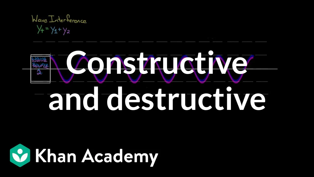
• Why this video: This video provides an intuitive and visual breakdown of wave superposition. Understanding how phase differences dictate whether waves reinforce or cancel each other out is critical, as this is the exact physical mechanism used by radio interferometers to combine signals.

---

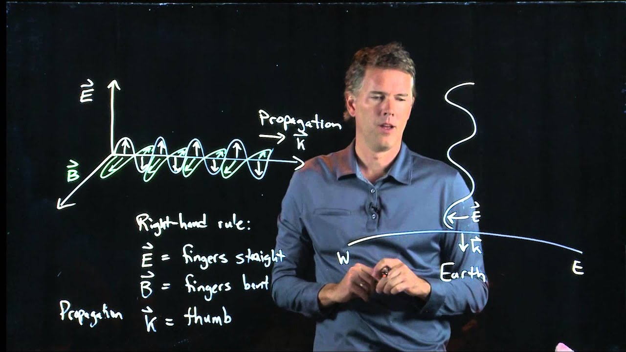
• Why this video: An exceptional lecture on James Clerk Maxwell’s unification of electricity and magnetism. It visualizes how self-propagating electric and magnetic fields create electromagnetic waves. This is vital for understanding the radio regime of the electromagnetic spectrum.

---

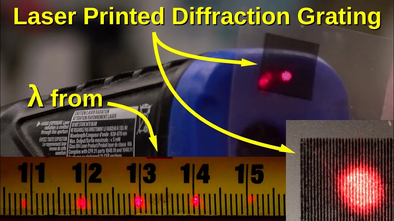
• Why this video: This video uses animated slit-experiment diagrams to demonstrate wave propagation and interference. It connects physical path differences directly to observable spatial interference patterns, laying the groundwork for baseline calculations in radio arrays.

---

Knowledge Checkpoint

• Define the principle of superposition and state the mathematical criteria for complete constructive and destructive interference.
• Calculate the path-length difference required to produce a phase shift of $\pi$ radians ($180^\circ$) for a radio wave of frequency $1.4\text{ GHz}$.
• Explain how electromagnetic waves propagate through space without a physical medium.

---

Module 2: Fundamentals of Radio Astronomy & Single Dish Telescopes

Before linking multiple dishes together, you must understand how a single radio telescope collects, focuses, and measures signal intensity. This module covers the mechanical operation of radio dishes and the physical limits of angular resolution imposed by the diffraction limit.

Deep-Dive: The Physics of the Diffraction Limit

For any circular aperture of diameter $D$ observing light at a wavelength $\lambda$, the minimum angular separation $\theta$ at which two distinct point sources can be resolved is governed by the Rayleigh Criterion:

$\theta \approx 1.22 \frac{\lambda}{D}$

This limit arises from the diffraction pattern (specifically, the Airy disk) created as incoming plane waves pass through the circular aperture. The factor of $1.22$ is derived from the first zero of the first-order Bessel function of the first kind $J_1(\pi \theta D / \lambda)$.

Because radio wavelengths are thousands to millions of times longer than optical light (e.g., $\lambda = 21\text{ cm}$ vs. $\lambda = 500\text{ nm}$), a single radio dish must be impractically large to resolve fine details. For example, to match the resolution of a modest $20\text{ cm}$ backyard optical telescope ($\approx 0.6$ arcseconds) at a $21\text{ cm}$ wavelength, a single radio dish would need to be over $70\text{ km}$ wide!

Recommended Videos

• Why this video: An in-depth primer that provides a complete overview of the radio sky, the mechanical and electronic construction of radio dishes, and how they detect astronomical phenomena.

---

• Why this video: This video features high-quality optical demonstrations and visual explanations of Rayleigh's criterion. It shows how diffraction patterns alter our ability to resolve individual sources as aperture size and wavelength change.

---

• Why this video: This tutorial directly links the math of angular resolution to practical observation, explaining the point spread function (PSF) and how single apertures blur point sources.

---

Knowledge Checkpoint

• Calculate the angular resolution (in arcseconds) of the $100\text{-meter}$ Effelsberg radio telescope observing at a wavelength of $6\text{ cm}$.
• Describe the path of an incoming radio wave from the reflecting surface of a parabolic dish to the receiver.
• Explain why a mesh surface can act as a perfect mirror for radio waves, provided the mesh spacing is much smaller than the observing wavelength ($\approx \lambda/10$).

---

Module 3: Principles of Radio Interferometry

Instead of building a single gargantuan dish, radio astronomers combine signals from smaller, physically separated telescopes. This module explains the physics of a basic two-telescope interferometer, the concept of baseline vectors, and the geometric principles of spatial frequency mapping.

Recommended Videos

• Why this video: Part of UC Berkeley's radio astronomy lecture series, Professor Aaron Parsons provides a clear, mathematically sound introduction to how two dishes act as a single interferometer. He shows how baseline vector geometry dictates the instrument's resolving power.

---

• Why this video: A short, high-density visualization of the geometric baseline ($B_{12}$) separating two dishes. It explains how this physical distance acts as a spatial filter on the sky.

---

• Why this video: This video introduces the $u\text{-}v$ plane, explaining how the baseline vector is projected from three-dimensional space onto a coordinate system perpendicular to the target source.

---

Knowledge Checkpoint

• Define the term "baseline" in the context of an interferometer. How does baseline length relate to the synthesized resolution?
• Explain how a geometric delay ($\tau_g = \vec{B} \cdot \hat{s} / c$) arises when a wavefront hits one antenna before another.
• Map the physical coordinates of a two-antenna baseline to a single point in the Fourier-space $u\text{-}v$ plane.

---

Module 4: Aperture Synthesis and Image Reconstruction

To create high-fidelity images, an interferometer must map as much of the $u\text{-}v$ plane as possible. This module explains how the Earth's natural rotation changes the projected baseline geometries over time (Earth rotation synthesis) and how mathematical algorithms convert these sparse spatial frequencies into a coherent image.

Deep-Dive: Earth Rotation Synthesis & the $u\text{-}v$ Plane

As the Earth rotates, the orientation of a physical baseline vector changes relative to the astronomical source. The coordinates $u$ and $v$ represent the baseline projected onto a plane perpendicular to the direction of the source:

$u = \frac{B_x}{\lambda} \sin H + \frac{B_y}{\lambda} \cos H$

$v = -\frac{B_x}{\lambda} \sin \delta \cos H + \frac{B_y}{\lambda} \sin \delta \sin H + \frac{B_z}{\lambda} \cos \delta$

Where:

• $B_x, B_y, B_z$ are the terrestrial baseline components.
• $H$ is the Hour Angle of the source (which changes continuously as Earth rotates).
• $\delta$ is the source declination.

Over a 12-to-24-hour observation run, this projection causes each antenna pair to trace out a semi-elliptical track in the $u\text{-}v$ plane. This naturally fills in the gaps of our virtual aperture.

u-v Plane (Spatial Frequencies) Reconstructed Image | +v /\ * * | * * / \ * | * | * | <-- Synthesized * | * Fourier | | Source Detail -----------+----------- Transform \ / * | u * ------------> \ / * | * \/ * * | * * | -v (Elliptical tracks traced by rotating baselines)

Deep-Dive: The CLEAN Algorithm

An interferometer sampling a sparse $u\text{-}v$ plane produces a highly distorted "dirty image" convolved with a "dirty beam" (the instrument's Point Spread Function, featuring massive sidelobes). Developed by Jan Högbom in 1974, the CLEAN algorithm deconvolves these components:

1. Find the Peak: Locate the brightest pixel in the dirty image.
2. Subtract a Fraction: Subtract a scaled version of the dirty beam (multiplied by a "loop gain" $\gamma \approx 0.1$) centered on that peak.
3. Record the Component: Save the location and subtracted amplitude of this "clean component" to a model list.
4. Iterate: Repeat steps 1–3 on the residual dirty image until the remaining noise reaches a specified threshold.
5. Reconstruct: Convolve the list of clean components with an idealized, smooth Gaussian "clean beam" (which lacks sidelobes) and add the final residual noise map back in to produce the final science-ready image.

Recommended Videos

• Why this video: An elegant visualization of how an array of radio antennas samples individual spatial frequencies. It shows how the Fourier transform bridges the $u\text{-}v$ plane and the final sky brightness distribution.

---

• Why this video: This video explains how the CLEAN algorithm deconvolves the dirty beam from raw, incomplete interferometric data to yield a high-fidelity image.

---

• Why this video: While part of a vintage dramatic production, this clip showcases the physical layout of an east-west baseline array. It provides a visual sense of how physical arrays are mechanically arranged to harness Earth's rotation.

---

Knowledge Checkpoint

• Explain how a pair of static, ground-based radio dishes can sweep out a continuous curve in the $u\text{-}v$ plane over 12 hours.
• Differentiate between a "dirty image" and a "clean image" in radio astronomy.
• Describe the function of the "loop gain" parameter ($\gamma$) in the CLEAN algorithm and the consequences of setting it too high or too low.

---

Module 5: Global Networks: VLBI and the Event Horizon Telescope

This capstone module covers Very Long Baseline Interferometry (VLBI). You will learn how global arrays synchronize separate observatories using atomic clocks to create an Earth-sized virtual telescope. This technique enabled the Event Horizon Telescope to capture the first historic image of a supermassive black hole.

Recommended Videos

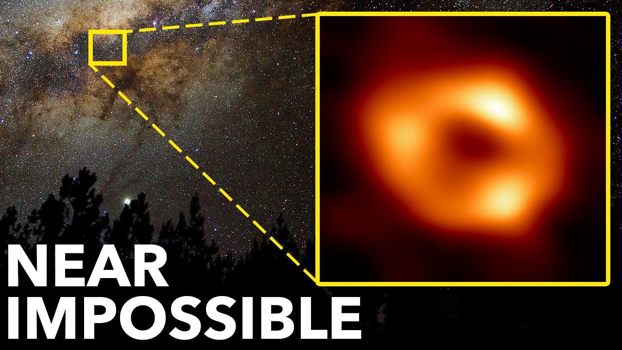
• Why this video: A masterpiece of science communication. Derek Muller walks through the mechanics of VLBI, demonstrating how telescopes across the globe record data to hard drives and use hydrogen maser atomic clocks to synchronize signals at a central correlator.

---

• Why this video: VLBI requires timing precision to within a fraction of a wave cycle (picoseconds). This video explains how atomic transitions in cesium and hydrogen maser clocks generate the ultrastable references needed to correlate global signals.

---

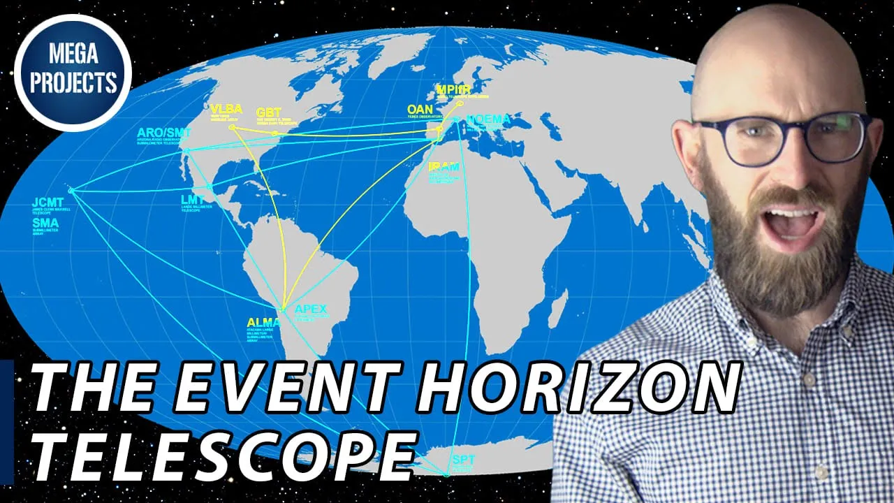
• Why this video: This video details the logistical and technical challenges of the Event Horizon Telescope campaign. It covers the extreme dry-altitude sites, data recording constraints, and the global coordination required to image M87* and Sgr A*.

---

Knowledge Checkpoint

• Explain why real-time fiber connections are impossible for global VLBI, and how hydrogen maser atomic clocks solve this synchronization problem.
• Estimate the angular resolution of a VLBI network operating at $1.3\text{ mm}$ wavelength with a maximum baseline of $10,700\text{ km}$ (approximate diameter of the Earth).
• Explain how a correlator combines data from different VLBI stations to reconstruct the mutual coherence of the electromagnetic field.

---

Course Map

---

Key People Index

• James Clerk Maxwell (1831–1879): Unified electricity and magnetism mathematically, proving that light is an electromagnetic wave.
• Lord Rayleigh (John William Strutt) (1842–1919): Established the fundamental limit of angular resolution for circular apertures.
• Jan Högbom (1929–Present): Invented the CLEAN algorithm in 1974, which revolutionized radio astronomy by allowing image reconstruction from sparse interferometric data.
• Katie Bouman (1989–Present): Led the development of imaging algorithms (like CHIRP) within the EHT collaboration that helped reconstruct the first-ever image of a black hole's shadow.

---

Final Self-Assessment

Complete this comprehensive test to evaluate your mastery of radio interferometry and global aperture synthesis:

• I can write and explain the wave superposition equation for two signals with a phase offset $\Delta \phi$.
• I can explain why radio telescopes need to be vastly larger than optical telescopes to achieve comparable angular resolution.
• I can calculate the angular resolution of an array given its maximum baseline and operating frequency.
• I can define the geometric delay ($\tau_g$) and explain how it is compensated for in an interferometer's correlator.
• I can draw or map how a baseline vector projects onto the $u\text{-}v$ plane.
• I can describe the mathematical link (Fourier Transform) between the visibility function $V(u,v)$ and the actual sky brightness distribution $I(l,m)$.
• I can outline the step-by-step process of the CLEAN algorithm, from the dirty image to the final convolved model.
• I can explain how the Earth's rotation acts to fill the $u\text{-}v$ plane over time.
• I can describe how VLBI records data locally using atomic clocks and why this data must be correlated retrospectively.
• I can identify the key scientific achievements of the Event Horizon Telescope regarding M87* and Sgr A*.