In radio interferometry, telescopes like ALMA do not directly capture images but instead measure the Fourier transform of a source's intensity distribution; this transform consists of amplitude values (indicating how many pieces of each spatial frequency exist) and phase values (indicating how to assemble them), with the number and spacing of antennas determining which spatial frequencies can be recorded, and the Fourier transform of a Gaussian distribution being another Gaussian where width in the sky corresponds inversely to width in the Fourier plane.
ALMA Explained: Fourier Transform in Interferometry
Added:Deep Dive
Basic wave mechanics, including phase, amplitude, and constructive or destructive wave interference.
![[Vật Lý 11] Giao Thoa Sóng Cơ - Chương Trình Mới - Dễ Hiểu Nhất | Thầy VNA](https://i.ytimg.com/vi/pF0VuOenFxQ/maxresdefault.jpg)
[Vật Lý 11] Giao Thoa Sóng Cơ - Chương Trình Mới - Dễ Hiểu Nhất | Thầy VNA
143K
The amplitude at point M is AM = |2A cos(π(d1 - d2)/λ)|, where the absolute value ensures amplitude is positive. The amplitude reaches maximum AMmax = 2A when cos(π(d1 - d2)/λ) = ±1, occurring when π(d1 - d2)/λ = kπ (k is integer). This represents constructive interference where waves reinforce completely. The amplitude reaches minimum AMmin = 0 when cos(π(d1 - d2)/λ) = 0, occurring when π(d1 - d2)/λ = π/2 + kπ. This represents destructive interference where waves cancel completely. A point M oscillates with maximum amplitude when the path difference equals an integer multiple of wavelength: d1 - d2 = kλ (k ∈ Z). A point M oscillates with minimum amplitude when the path difference equals a half-integer multiple: d1 - d2 = (k + 1/2)λ (k ∈ Z).
Click to watch →

Wave Optics Class 12 Physics - 12 Marks in One Day🔥| Class 12 Physics Chapter 10 | NEET |Gaurav Sir
151.5K
Interference occurs when two waves superpose. Phase difference determines interference type: 0° causes constructive interference (amplitude adds), 180° causes destructive interference (amplitude subtracts). The net amplitude formula A_net² = A1² + A2² + 2A1A2cosφ applies universally. For constructive interference (φ=0°), A_net = A1 + A2; for destructive (φ=180°), A_net = |A1 - A2|. Intensity is proportional to amplitude squared (I ∝ A²). Net intensity formulas are I_net = (√I1 + √I2)² for constructive and I_net = (√I1 - √I2)² for destructive. When amplitudes are equal, constructive gives 4I0 and destructive gives 0.
Click to watch →

Wave Optics (तरंग प्रकाशिकी) | UP Board 2022 | Physics One Shot Revision | भौकाल Batch
10K
When two light waves superpose: (1) Constructive interference (sustaining interference) occurs when waves meet in phase, resulting in increased amplitude and intensity, (2) Destructive interference (annihilating interference) occurs when waves meet out of phase, resulting in decreased or zero amplitude and intensity. The resultant wave depends on the phase relationship between the two interfering waves. The phase difference determines whether interference is constructive or destructive.
Click to watch →

Waves -One Shot l NCERT Physics Class 11 chapter 15 l Wave motion ll CBSE ll NEET II Mechanical Wave
65.1K
Constructive interference occurs when waves meet in phase (phase difference = 0, 2π...), resulting in maximum amplitude (2A). Destructive interference occurs when waves meet out of phase (phase difference = π, 3π...), resulting in minimum or zero amplitude. The resultant amplitude depends on the phase difference between the waves.
Click to watch →

اقوى ورشة عمل للصف الثاني الثانوي "مراجعة مارس" | م.محمود مجدي 💪❤️
95.7K
Key wave characteristics include: (1) Amplitude: maximum displacement from equilibrium position, (2) Wavelength (λ): distance between consecutive crests or troughs, or twice the distance between a crest and trough, (3) Phase: the position and direction of a point on the wave at a given time. Two points are in phase if they have the same displacement and direction of motion.
Click to watch →
Deep Dive
The fundamental principles of radio astronomy and how antennas detect electromagnetic radiation rather than optical light.

3rd USNC-URSI E-Lecture: Our Electromagnetic Window on the Universe | Dr. David DeBoer
796
Radio waves are electromagnetic radiation at longer wavelengths than visible light, with wavelength and frequency coupled by the speed of light. Wavelength determines antenna size requirements, while frequency determines sampling rates. Unlike optical astronomy which primarily measures amplitude, radio astronomy can measure both amplitude and phase, enabling interferometry and high-resolution imaging. The ionosphere blocks frequencies below 10 MHz, limiting ground-based observations. Different frequencies probe different physical processes in the universe, with radio waves revealing cooler objects and non-thermal radiation that optical astronomy cannot detect.
Click to watch →

Radio Astronomy from Space by Dr. Mayuri Rao
153
Radio astronomy studies the universe using radio waves, which occupy the lowest energy scales in the electromagnetic spectrum (megahertz to terahertz). Unlike optical telescopes that detect photons with cameras, radio telescopes use antennas to detect waves, enabling coherent detection that provides both amplitude and phase information. Key measurements include specific intensity (intrinsic source brightness) and flux density (power received, decreasing with distance squared). The Jansky unit (10⁻²⁶ W/m²/Hz) measures flux density, with sensitive surveys detecting microJansky signals.
Click to watch →

An Introduction to Radio Astronomy
570
Radio astronomy studies celestial objects using radio waves, which are a different color of light invisible to the naked eye. The basic process involves transmitters converting signals to electricity, antennas radiating signals, and receivers converting them back. The Jansky unit (10^-26 watts per square meter per hertz) measures signal strength, which is incredibly weak. The electromagnetic spectrum ranges from gamma rays to radio waves, with radio waves generated by oscillating charges. Temperature determines radiation type - hotter objects emit higher energy radiation. Radio waves pass through Earth's atmosphere without attenuation, unlike visible light. Induction occurs when magnetic field lines pass through conductive materials, producing electricity. Loop antennas detect electromagnetic radiation by inducing current, with polarization affecting signal strength.
Click to watch →

Optics in Space by Dr. B. Vishweshwar Rao
4.2K
Radio astronomy fundamentally differs from optical astronomy in detection methodology. While optical telescopes detect individual photons using cameras and CCD sensors, radio astronomy senses coherent wave packets where amplitude and phase can both be measured. Specific intensity represents an intrinsic source property independent of distance, while flux density—the measured quantity—decreases with the square of distance. The Jansky (10^-26 W/m²/Hz) serves as the standard unit for radio flux density, with modern telescopes achieving sensitivities down to microjanskys. Antenna gain relates to effective area and wavelength, while angular resolution depends on wavelength and aperture size. Interferometry enables astronomers to create effectively larger telescopes by combining signals from multiple smaller antennas, producing interference patterns containing spatial frequency information. The visibility function and intrinsic sky brightness share a Fourier transform relationship, enabling reconstruction of high-resolution images through inverse Fourier transformation.
Click to watch →

Radio Astronomy and the hunt for radio stars
239
Radio astronomy studies radio waves as electromagnetic light, not sound. The electromagnetic spectrum includes gamma rays, X-rays, UV, visible light, infrared, microwaves, and radio waves. Radio waves have wavelengths from centimeters to meters, much longer than visible light (hundreds of nanometers). Radio waves penetrate dust and gas that block visible light, allowing observation of the galactic center. Thermal radiation is created by heat, while non-thermal synchrotron radiation is created when charged particles spiral through magnetic fields. Optical telescopes count individual photons, while radio telescopes detect electrical signals induced in wires when waves pass over them.
Click to watch →
Deep Dive
A conceptual understanding of the Fourier Transform and its role in translating signals between the spatial domain and the frequency domain.
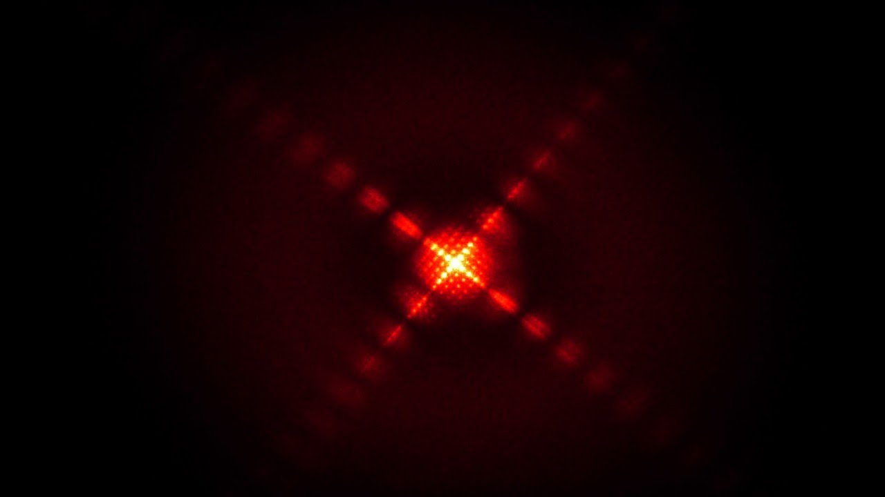
Intro to Fourier Optics and the 4F correlator
153.6K
The Fourier transform converts signals between time/frequency domains and spatial frequency domains. In time domain, sine waves produce single frequency spikes, square waves reveal harmonics, and noisy signals show distributed noise. For spatial images, sine wave intensity patterns transform into symmetric dot pairs, while square waves produce multiple dots at decreasing intensities representing harmonics. Natural images show bright central spots surrounded by random noise due to complex frequency combinations. Crucially, magnitude-only Fourier transforms lose phase information, meaning feature location doesn't affect the output - identical features at different positions produce identical frequency domain representations.
Click to watch →
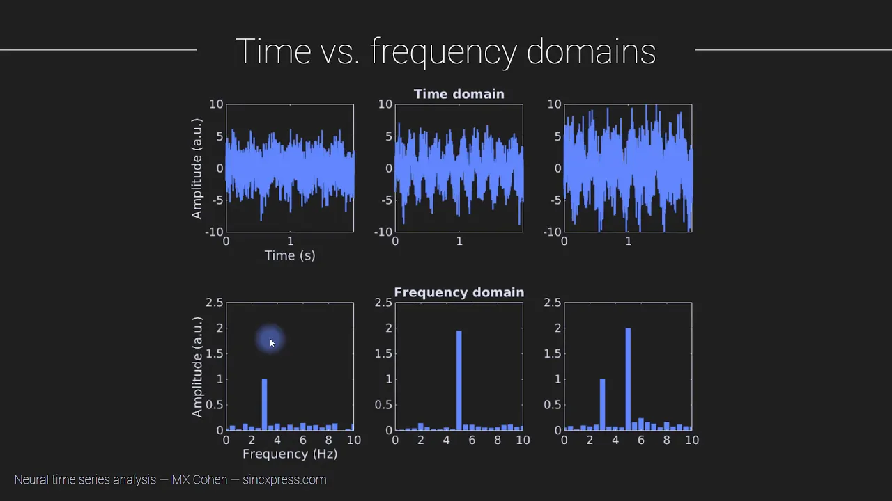
Time and frequency domains
123.5K
The frequency domain offers critical advantages for signal analysis, particularly with noisy data. Random noise (white noise) appears as broadband components with low amplitude in the frequency domain, while actual sinusoidal components remain as distinct, prominent peaks. This occurs because white noise has a flat power spectrum—small contributions at many frequencies sum to substantial noise in the time domain, but remain individually visible in the frequency domain. Understanding the Fourier transform requires building knowledge progressively from three foundations: sine waves as periodic signal building blocks, complex numbers for representing magnitude and phase, and the dot product for measuring vector similarity. These combine to form complex sine waves and complex dot products, which together yield Fourier coefficients representing each frequency component's amplitude and phase. This systematic approach enables complete understanding of spectral analysis techniques.
Click to watch →
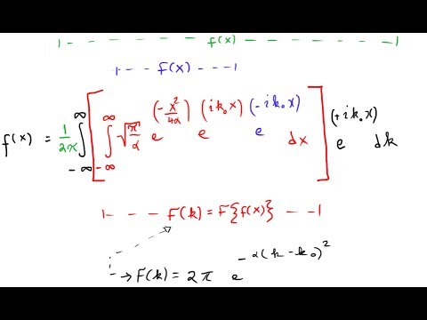
The Fourier Transform in 15 Minutes
520.1K
The Fourier transform converts a function from one domain to another. When you input a function of time (measured in seconds), the output is a function of frequency (measured in Hz). Similarly, if you input a function of position (meters), the output is a function of spatial frequency (per meter). This transformation changes the basis of your function from time/space to frequency/spectral components.
Click to watch →

What is the Fourier Transform? ("Brilliant explanation!")
200.9K
The Fourier Transform is a mathematical tool that converts a signal from the time domain to the frequency domain, representing any signal as a sum of sinusoidal components at different frequencies. A pure cosine wave at frequency f₁ transforms to two delta functions at +f₁ and -f₁ on the frequency axis, each with amplitude 0.5, because cosine can be expressed as the sum of two complex exponentials (positive and negative frequencies). Similarly, a sine wave at the same frequency requires the same frequency components but with different phase relationships: the positive frequency component has a phase of -π/2 and the negative frequency component has a phase of +π/2. This demonstrates why complex numbers are essential in the Fourier Transform—they allow us to capture both amplitude and phase information needed to distinguish between sine and cosine signals at the same frequency.
Click to watch →
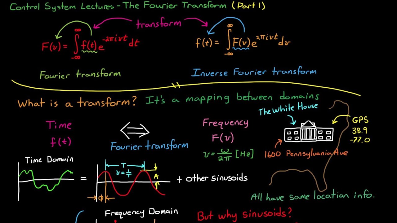
Introduction to the Fourier Transform (Part 1)
1.6M
The Fourier Transform is a mathematical operation that converts functions between time and frequency domains. The forward transform converts time-domain signals f(t) to frequency-domain representations F(ω), while the inverse transform reverses this process. A transform is fundamentally a mapping between different data domains, similar to describing a location using different address formats - all contain the same information but in different forms. Fourier's discovery in the early 18th century revealed that any continuous signal can be represented as a sum of sinusoids, each characterized by amplitude, frequency, and phase. This decomposition is powerful because sinusoids maintain their shape through Linear Time-Invariant systems, allowing engineers to analyze system behavior through amplitude and phase changes at each frequency.
Click to watch →
Deep Dive
The basic concept of astronomical interferometry and why multiple physically separated telescopes are used together to act as a single large instrument.

Using Jupiter's Lagrange Points, JWST Staying in Place, Fighting Mars' Low Gravity | Q&A 289
47K
Interferometry is a technique where multiple telescopes separated by large distances work together to function as a single, much larger telescope. The resolving power of an interferometer equals the distance between its component telescopes rather than their individual sizes. The Event Horizon Telescope used this principle by linking radio telescopes around the world to create an Earth-sized virtual telescope that captured images of black hole event horizons. However, visible light interferometry faces significant challenges because wavelengths are too short (nanometers) to align precisely over large distances. Tidal flexing of the Earth and atmospheric disturbances make perfect alignment impossible beyond a few hundred meters. Space-based interferometers could overcome these limitations by maintaining precise distances between free-floating telescopes using laser ranging, potentially creating telescopes spanning tens to thousands of kilometers.
Click to watch →

DEEP Space Documentary
131.4K
Interferometry takes light from two separate telescopes and brings it together in a single point while preserving the relative shifts between light waves. If done precisely, the two telescopes act as if they were part of a single colossal mirror as large as the distance between them. This gives smaller telescopes the resolving power of a much larger instrument. The twin Keck telescopes on Mauna Kea regularly team up as an interferometer, while the VLT can have four telescopes working together. Major modern telescopes include Subaru and Gemini North on Mauna Kea, Gemini South in Chile, the Magellan telescopes in Chile, and the Large Binocular Telescope in Arizona. They are constructed at the best available sites—high, dry, clear, and dark—with mirrors as large as swimming pools, all equipped with adaptive optics to counteract atmospheric blurring. For over two centuries, astronomers had to be artists, peering through eyepieces and making detailed drawings of what they saw, but sometimes over-interpreting what they saw, such as dark linear features on Mars that were thought to be canals suggesting civilized life.
Click to watch →
E se os ALIENÍGENAS ESTIVEREM NOS OBSERVANDO?
31.1K
Interferometry is a technique that overcomes telescope size limitations by combining multiple smaller telescopes to function as a single virtual telescope. The ALMA (Atacama Large Millimeter Array) uses multiple radiotelescopes working together to create a virtual telescope 16 kilometers in diameter. This same technique was used by the Event Horizon Telescope team to capture the first image of a black hole in 2019, using seven radiotelescopes worldwide to create a virtual telescope spanning Earth's diameter.
Click to watch →

IT'S FINALLY HAPPENED... WE'RE LIVE!
40K
Interferometry combines multiple small telescopes to achieve the resolution of a single large telescope. The hosts explain that radio astronomy uses this technique by combining signals from multiple radio telescopes to achieve high resolution. The resolution of a telescope is determined by the ratio of its diameter to the wavelength of light, so combining multiple small telescopes can achieve the resolution of a much larger single telescope. The hosts also discuss optical interferometry, which is more challenging due to the shorter wavelengths requiring extremely precise alignment and phasing.
Click to watch →

Як інтерферометри здатні бачити найдрібніші деталі космічних об'єктів?
28.9K
Interferometry is an astronomical technique that combines signals from multiple smaller telescopes to achieve the resolution of a much larger virtual telescope, where the effective diameter equals the distance between the individual telescopes; this method overcomes the physical limitations of single large telescopes, which suffer from gravitational deformation and technical challenges at scales beyond 5 meters, enabling astronomers to observe fine details of celestial objects like protoplanetary disks and black holes that would otherwise be impossible to resolve.
Click to watch →
Prerequisite Knowledge
- Concept 01Basic wave mechanics, including phase, amplitude, and constructive or destructive wave interference.
- Concept 02The fundamental principles of radio astronomy and how antennas detect electromagnetic radiation rather than optical light.
- Concept 03A conceptual understanding of the Fourier Transform and its role in translating signals between the spatial domain and the frequency domain.
- Concept 04The basic concept of astronomical interferometry and why multiple physically separated telescopes are used together to act as a single large instrument.
Subsequent Learning
- Step 01The concept of the 'uv-plane' and aperture synthesis, detailing how physical telescope arrangements sample spatial frequencies.
- Step 02Deconvolution techniques in radio astronomy, such as the CLEAN algorithm, used to reconstruct true cosmic images from incomplete Fourier data.
- Step 03Phase calibration and self-calibration methods used to correct for atmospheric distortions that alter radio wave phases.
- Step 04Advanced applications of interferometry, such as Very Long Baseline Interferometry (VLBI) and the imaging techniques used by the Event Horizon Telescope.
Fourier Basics
Visibility Cases
Fourier Basics
0:08Playing Section
- 1
Interferometers sample the source's Fourier transform, not direct images.
- 2
Amplitude indicates component sizes; phase reveals how to assemble them.
- 3
Limited antenna pairs restrict spatial frequency coverage and reconstruction quality.
Regularized Maximum Likelihood (RML) and Compressive Sensing
While traditional interferometry relies on the Fourier transform and the CLEAN algorithm to reconstruct images from gridded visibility data, this classical approach struggles with highly incomplete or sparse data. An increasingly prominent alternative paradigm uses Regularized Maximum Likelihood (RML) and Compressive Sensing (CS) techniques. Instead of performing a direct inverse Fourier transform on gridded data and then deconvolving, RML methods define an image grid directly and use optimization algorithms to find the image that best fits the observed visibilities. By incorporating mathematical priors such as sparsity, smoothness, or maximum entropy, RML can reconstruct images without the artificial bias or 'dirty beam' artifacts introduced by traditional Fourier gridding. This alternative approach, notably championed by the Event Horizon Telescope to image black holes, represents a shift from classical transform-based reconstruction to forward-modeling optimization, offering superior resolution and artifact suppression in sparse interferometric arrays.
Deep Dive
The concept of the 'uv-plane' and aperture synthesis, detailing how physical telescope arrangements sample spatial frequencies.
The Van-Cittert Zernike theorem and the image-object relation
4.8K
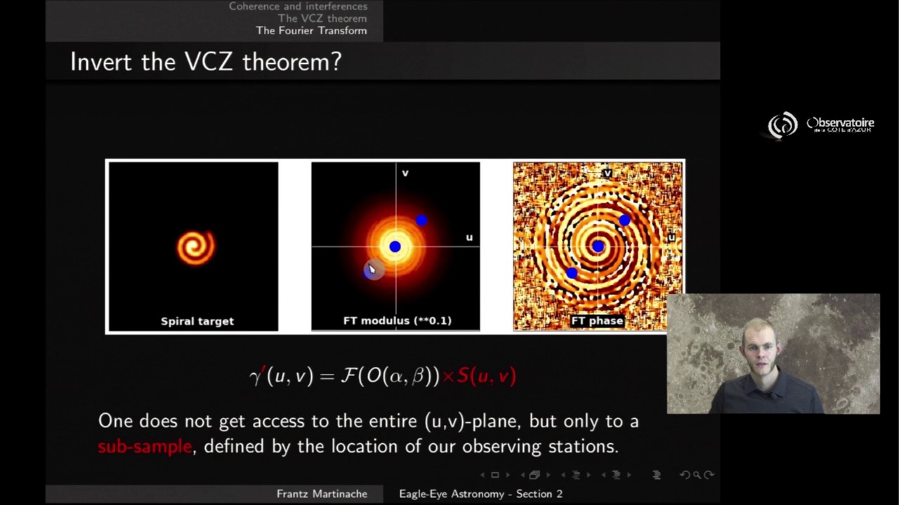
Practical interferometry faces fundamental limitations: the infinite UV plane cannot be fully sampled. Observing station locations determine discrete sampling points. Two-aperture systems sample single points, while three-aperture configurations produce triangular patterns with three distinct sampling locations. The autocorrelation function of the pupil map mathematically describes these sampling patterns, showing how aperture arrangements create characteristic UV coverage that constrains astronomical reconstructions.
Click to watch →

ANITA Lecture - Radio Astronomy and Interferometry Fundamentals – David Wilner
29.3K
The visibility function reveals source structure through its dependence on baseline orientation and length. At the UV origin, visibility equals total flux density. Point sources produce constant visibilities regardless of baseline orientation, while resolved sources show varying visibilities as different baseline angles sample different portions of the source structure. Aperture synthesis reconstructs the full sky brightness by sampling the visibility function across the UV plane using multiple antenna configurations. Earth rotation naturally fills the UV plane over time, and multiple wavelength observations can cover different spatial frequencies simultaneously. The technique requires sufficient UV coverage to satisfy the sampling theorem and assumes the source remains static during observation.
Click to watch →
Как радиотелескоп видит чёрные дыры и всё остальное?
52.2K
In aperture synthesis, radio astronomers construct a spatial frequency plane where different frequencies correspond to different scales of detail in the final image. A filled-aperture telescope (like optical telescopes) can observe all spatial frequencies simultaneously, producing complete images. However, interferometers with multiple antennas can only observe specific spatial frequencies corresponding to the baselines between pairs of antennas. This means an interferometer with two antennas can only see details of a particular size range—similar to seeing only pimples but not freckles or hair in a portrait photograph.
Click to watch →

Stella Offner "Performing Synthetic Interferometric Observations with CASA"
168
Aperture synthesis combines signals from multiple antennas to produce an image with resolution equivalent to a single antenna spanning the entire array. The quality of the resulting image depends critically on UV plane sampling—the distribution of baseline vectors traced during observations. Better sampling (more points in the UV plane) enables better Fourier reconstruction and improved image quality. Observers increase sampling by using more antennas and taking advantage of Earth's rotation, which changes the projected baselines over time. Insufficient sampling results in incomplete UV coverage, leading to poor image reconstruction and artifacts.
Click to watch →

Radio Interferometry II: Fringe Patterns & UV Plane Sampling
5.7K
The UV plane is the Fourier transform domain where interferometric data is processed. It transforms sky coordinates (L, M) into baseline coordinates (U, V). Each antenna pair samples a specific point in the UV plane based on their separation vector. The UV plane contains all spatial frequency information needed to reconstruct the original sky image through inverse Fourier transformation.
Click to watch →
Deep Dive
Deconvolution techniques in radio astronomy, such as the CLEAN algorithm, used to reconstruct true cosmic images from incomplete Fourier data.

ANITA Lecture - Imaging and Deconvolution in Radio Interferometry – David Wilner
13.6K
Due to missing UV samples, infinitely many sky brightness distributions are compatible with measured visibilities, making the true sky brightness non-unique. The CLEAN algorithm assumes point sources and iteratively identifies peaks in the residual map, subtracts scaled dirty beams, and accumulates clean components. Variants like multiscale CLEAN use broader Gaussians for extended emission. No unique optimum solution exists—different approaches yield different scientifically valid results. After CLEAN completes, a restored image combines clean components, convolved with a clean beam, plus residual noise. Missing short spacings (samples near UV plane center) cause loss of largest emission scales, reducing central brightness by half for Gaussian sources exceeding ~18 arcseconds at 100 GHz with 15-meter baseline. Solutions include single-dish telescopes measuring all visibilities from 0 to D (dish diameter), then dividing out primary beam response, and compact arrays with smaller antennas filling the short spacing gap. ALMA implements this comprehensively: main array (12m antennas, 12m-14km baselines), compact array (7m antennas, 0-12m baselines), and single-dish antennas. The lecture concludes that interferometry samples Fourier components of sky brightness, imaging requires Fourier transforming sampled visibilities, but incomplete sampling creates an infinite number of compatible images, requiring scientific judgment in the imaging and deconvolution process to extract meaningful astronomical information.
Click to watch →

SMA School 2021: Imaging and Deconvolution
706
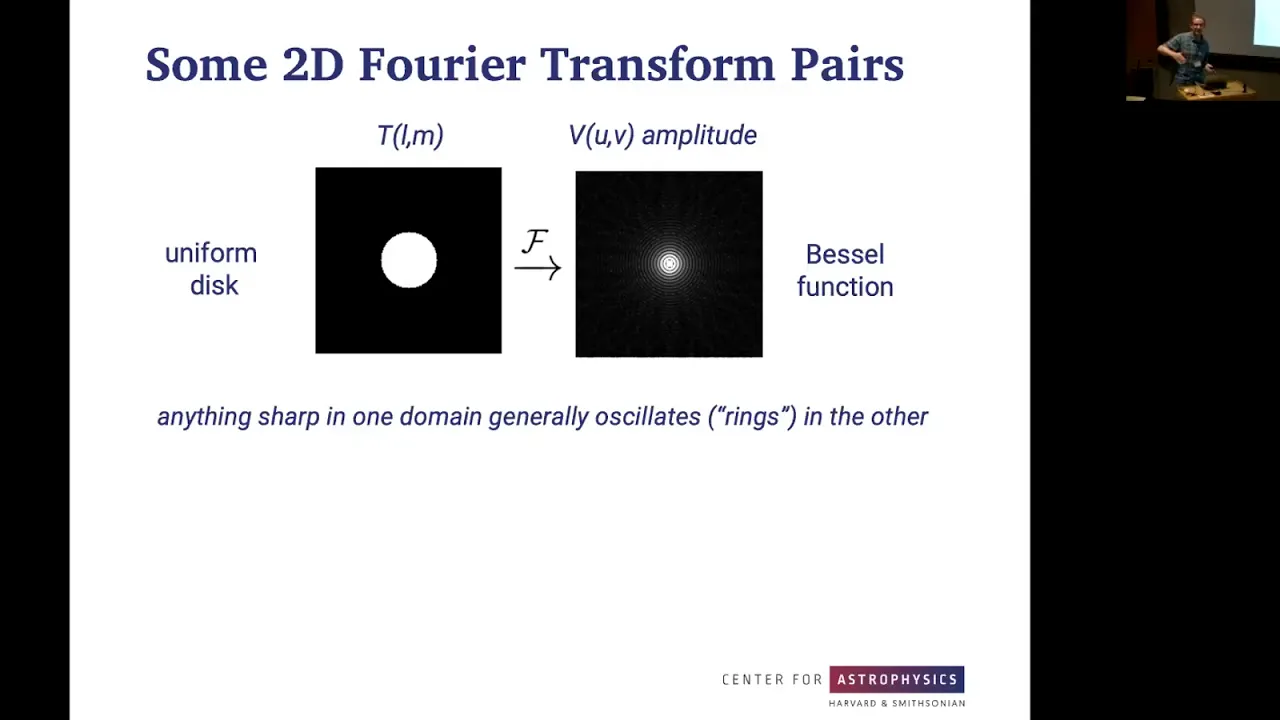
Radio interferometric imaging reconstructs astronomical images by taking the Fourier transform of sampled visibility data, where the visibility function V(u,v) represents the 2D Fourier transform of the sky brightness distribution T(l,m); however, because interferometers cannot sample the entire uv plane uniformly (creating gaps and missing short spacings), the resulting 'dirty image' is blurred by the synthesized beam, requiring deconvolution algorithms like CLEAN or Maximum Entropy to recover the true sky brightness distribution by iteratively removing the beam's influence and extrapolating the missing Fourier components.
Click to watch →
ALMA Primer: How the CLEAN Algorithm Deconvolves Interferometric Images
2.3K
The CLEAN algorithm, developed by Ronald Hogg in 1974, is the standard method for reconstructing astronomical images from radio interferometry data by iteratively deconvolving the dirty beam from dirty images; the algorithm works through nested major and minor cycles where minor cycles perform image-plane deconvolution to add clean components to the model, while major cycles transform back to the uv plane for accurate subtraction, balancing computational efficiency with image accuracy.
Click to watch →

Imaging and deconvolution 1080p
269
Radio interferometers measure the visibility function, which is the Fourier transform of the sky brightness distribution according to the Van Cittert-Zernike theorem; the relationship between visibility space and image space follows the convolution theorem, meaning convolution in one domain equals multiplication in the other. The interferometer's response to a point source is called the point spread function (PSF) or dirty beam, which appears as side lobes in the initial dirty image due to missing spatial frequency samples in the uv plane. The CLEAN algorithm removes these PSF artifacts through iterative subtraction of scaled PSFs from peak sources, producing a restored image. For two-dimensional arrays, the w-component introduces direction-dependent smearing that requires correction via faceting, w-projection, or w-stacking. Weighting schemes like natural, uniform, and robust weighting control the trade-off between sensitivity and resolution during image formation.
Click to watch →
SMA School 2020: Imaging and Deconvolution
127
Deconvolution algorithms address the fundamental challenge that infinitely many images match measured visibilities. CLEAN assumes sky consists of point sources: iteratively finds peaks, subtracts scaled dirty beams, adds to model, repeats until threshold (2-3× RMS noise). Restored image convolves model with clean beam and adds residuals. Maximum Entropy minimizes objective function combining data agreement and entropy, assuming smooth, positive sky. Both require assumptions about true sky structure. Dynamic range (peak brightness/RMS noise) provides reconstruction accuracy lower limit. Fidelity measures how closely reconstructed image matches truth. Large-scale structure problems arise from central hole in UV coverage (minimum baseline), potentially missing or distorting extended emission. For Gaussian sources, central brightness can be reduced by ~50% before apparent size changes significantly.
Click to watch →
Deep Dive
Phase calibration and self-calibration methods used to correct for atmospheric distortions that alter radio wave phases.

ALMA Primer Series: Intro to Calibration
972
The atmosphere introduces noise (sky temperature) and causes phase offsets/amplitude variations (gain fluctuations) due to ice structures, clouds, and water vapor density changes. Water vapor radiometers monitor variations every 1.1 seconds, applying corrections during pipeline processing. Phase calibrators—bright compact sources near science targets—are observed periodically; cadence depends on atmospheric stability, frequency, and baseline length (every 90 seconds for long baselines, 5-10 minutes for shorter ones). Self-calibration uses bright sources in the field to correct variations on timescales as short as seconds, significantly improving data quality when applied correctly.
Click to watch →
ALMA explained: ALMA calibration
426
ALMA data calibration involves correcting atmospheric and instrumental effects to achieve zero phases and flat amplitudes, using three types of calibrators: bandpass calibrators (quasars with flat spectra) for instrumental corrections, flux calibrators (monitored quasars or solar system objects) for converting arbitrary amplitudes to physical values, and gain calibrators (nearby point sources) for phase referencing to correct atmospheric effects, with self-calibration applied when amplitude variations occur over time.
Click to watch →
I-TRAIN #4: ALMA WebLog inspection
393
System temperature measures background emission from sky, telescope, and instrument, used for amplitude correction. Atmospheric transmission shows signal passage through the atmosphere—variations should be removed. Dips in transmission correspond to increased system temperature, expected behavior. WVR-based phase calibration uses water vapor radiometers to measure atmospheric water vapor and correct phase effects caused by atmospheric turbulence. Diagnostic plots compare phase RMS before and after correction—red wiggles should be much smaller than gray wiggles indicating successful correction. Orange lines indicate interpolated corrections for problematic antennas. Magenta lines show where calculations couldn't be applied. Bandpass solutions show amplitude versus frequency for each antenna—solutions should appear smooth but don't need to be perfectly flat. Sharp spikes indicate observation problems. Phase versus frequency plots may show small wiggles near zero, acceptable behavior.
Click to watch →

Self Calibration and Calibration 1080p
459
Self-calibration is an iterative calibration technique in radio astronomy where astronomers use the target field itself as a calibrator by creating an initial image, deriving a model, and then calibrating visibilities to that model, repeating the process to improve calibration quality; this addresses residual phase variations from atmospheric effects and electronic instabilities that persist after initial transfer calibration, with direction-dependent calibration extending this approach to correct for antenna-specific errors like primary beam variations and ionospheric effects that vary across the sky, requiring sophisticated tools like Cubicle and DDFacet to solve for different gain corrections for different patches of sky simultaneously.
Click to watch →

Govind Swarup Memorial Lecture 2024
489
Interferometry requires precise phase alignment for proper image reconstruction, as all waves must have maximum amplitude at the same point. Phase calibration involves adjusting instrument phases to achieve this alignment, with challenges from ionospheric and atmospheric variations. Self-calibration, developed by Conwell and Wilkinson, treats unknown phase errors as additional parameters to be solved alongside the image itself. For 30 telescopes with 435 measurements, this approach dramatically improves dynamic range (ratio of strongest source to noise) from designed 500 to tens of thousands. This technique represents a key advancement in handling phase instabilities in radio interferometry.
Click to watch →
Deep Dive
Advanced applications of interferometry, such as Very Long Baseline Interferometry (VLBI) and the imaging techniques used by the Event Horizon Telescope.

COMO FIZERAM A PRIMEIRA IMAGEM DE UM BURACO NEGRO PREVISTO POR EINSTEIN?
24.5K
VLBI is an interferometry technique where telescopes are located at widely separated points on Earth, sometimes thousands of kilometers apart. The Event Horizon Telescope (EHT) used VLBI to image the black hole in galaxy M87 by distributing radio telescopes across the globe, creating an effective aperture the size of Earth. The system uses known astronomical sources (quasars) to calibrate and measure distances between telescopes, combined with extremely precise atomic clocks to measure signal arrival times. This distributed approach allowed the EHT to achieve the resolution needed to image a black hole millions of light-years away.
Click to watch →
So sieht das Magnetfeld unseres Schwarzen Lochs aus!
49.1K
Very Long Baseline Interferometry (VLBI) is an astronomical technique that connects multiple radio telescopes across the globe to function as a single, enormous virtual telescope. By synchronizing these telescopes and combining their signals, astronomers create an effective telescope with a diameter approximately equal to Earth's diameter. In radio astronomy, larger telescope dishes provide higher resolution, and this technique enables the Event Horizon Telescope to achieve the extreme resolution necessary to image distant black holes that would be impossible to capture with any single telescope.
Click to watch →

The Large Millimeter Telescope
2.2K
The Event Horizon Telescope uses very long baseline interferometry by coordinating global radio telescopes. Each site records data with atomic clock timestamps, then combines signals later. Precise timing (fractions of nanoseconds) and GPS coordinates enable reconstruction of high-resolution images from widely-separated telescopes, effectively creating a virtual Earth-sized telescope for imaging black hole shadows.
Click to watch →
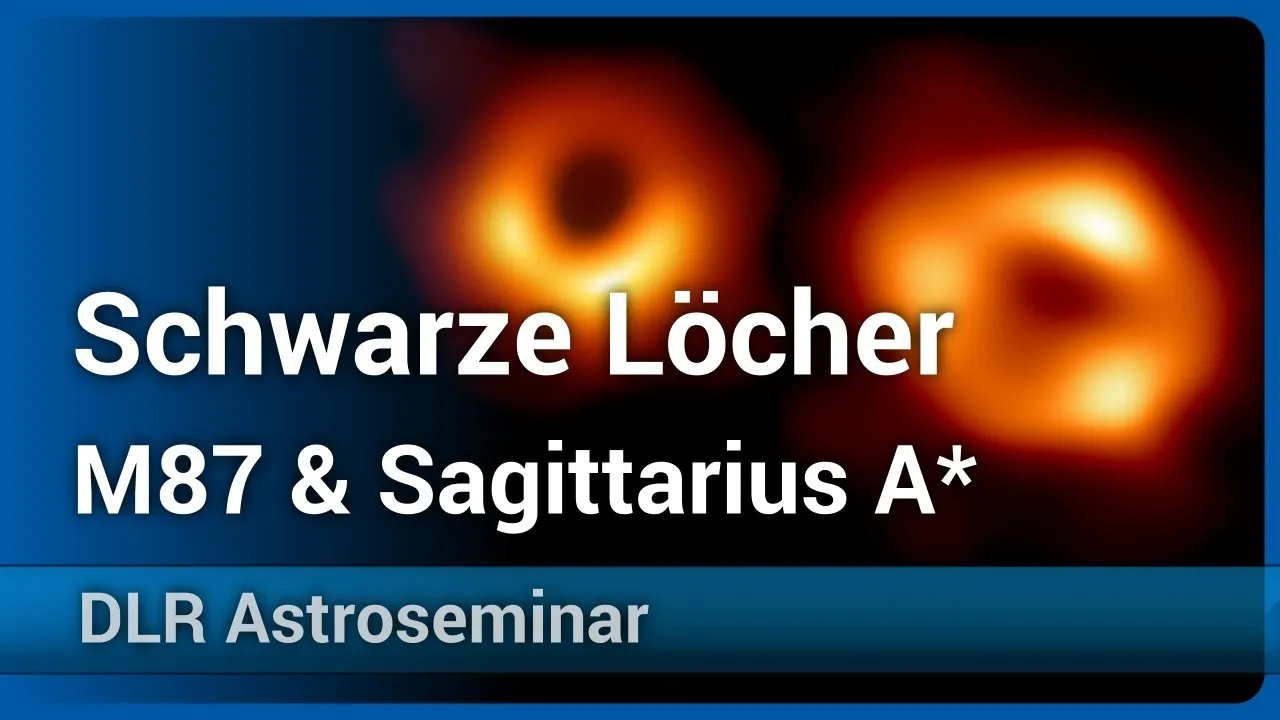
Schwarze Löcher M87 & Sagittarius A* • EHT • DLR Astroseminar | Heino Falcke
223.3K
The Event Horizon Telescope uses very-long-baseline interferometry (VLBI) to achieve the necessary resolution. This technique combines signals from multiple radio telescopes around the world, effectively creating an Earth-sized telescope. The telescopes record data with atomic clocks, and the data is later combined to produce images with the resolution of an Earth-sized aperture. The Earth's rotation provides additional baselines for interferometry measurements, allowing reconstruction of images from many different interferometric measurements.
Click to watch →

Chegou a Hora!!! Vamos Observar Um Buraco Negro - Space Today TV Ep.614
76.8K
The Event Horizon Telescope uses Very Long Baseline Interferometry (VLBI), a technique that combines radio telescopes from multiple continents to function as a single giant telescope. The ALMA observatory in Chile recently joined the project, increasing the telescope's sensitivity by a factor of 10. All telescopes are pointed at the same target, and their signals are combined at a central location to create the image.
Click to watch →
Fourier Basics
Visibility Cases
Fourier Basics
0:08- 1
Interferometers sample the source's Fourier transform, not direct images.
- 2
Amplitude indicates component sizes; phase reveals how to assemble them.
- 3
Limited antenna pairs restrict spatial frequency coverage and reconstruction quality.
Regularized Maximum Likelihood (RML) and Compressive Sensing
While traditional interferometry relies on the Fourier transform and the CLEAN algorithm to reconstruct images from gridded visibility data, this classical approach struggles with highly incomplete or sparse data. An increasingly prominent alternative paradigm uses Regularized Maximum Likelihood (RML) and Compressive Sensing (CS) techniques. Instead of performing a direct inverse Fourier transform on gridded data and then deconvolving, RML methods define an image grid directly and use optimization algorithms to find the image that best fits the observed visibilities. By incorporating mathematical priors such as sparsity, smoothness, or maximum entropy, RML can reconstruct images without the artificial bias or 'dirty beam' artifacts introduced by traditional Fourier gridding. This alternative approach, notably championed by the Event Horizon Telescope to image black holes, represents a shift from classical transform-based reconstruction to forward-modeling optimization, offering superior resolution and artifact suppression in sparse interferometric arrays.
Basic wave mechanics, including phase, amplitude, and constructive or destructive wave interference.
The fundamental principles of radio astronomy and how antennas detect electromagnetic radiation rather than optical light.
A conceptual understanding of the Fourier Transform and its role in translating signals between the spatial domain and the frequency domain.
The basic concept of astronomical interferometry and why multiple physically separated telescopes are used together to act as a single large instrument.
The concept of the 'uv-plane' and aperture synthesis, detailing how physical telescope arrangements sample spatial frequencies.
Deconvolution techniques in radio astronomy, such as the CLEAN algorithm, used to reconstruct true cosmic images from incomplete Fourier data.
Phase calibration and self-calibration methods used to correct for atmospheric distortions that alter radio wave phases.
Advanced applications of interferometry, such as Very Long Baseline Interferometry (VLBI) and the imaging techniques used by the Event Horizon Telescope.
1.1K views23likes3:02@europeanalmaregionalcentre2068Original Release: 2021-11-17
hi my name is sebastian and i am daniel we are both working at the nordicama regional center and in this short video we are going to talk about the fourier transform in interferometry when we look at a source in the sky with an interferometer like alma we do not get a direct image what we measure with an interferometer is some values of the fourier transform of the intensity distribution of the source the fourier transform is a mathematical concept it is a complex function with an amplitude and a phase let's take this brick assembly game as an analogy to try to understand what is happening without going into the mathematics take your object break it down into pieces of different sizes one piece would be one typical size so-called spatial frequency in your space which is measured by one pair of antennas roughly speaking the amplitude of the fourier transform will tell you how many pieces of each size you have in your image and the phase will contain information on how to assemble the pieces in principle we would need all the pieces to reconstruct the object but unfortunately we have a limited amount of antennas and we cannot register all the pieces if you put antennas too close you will not be able to see small pieces and you will lose resolution if you put your antennas far apart you start to lose the largest pieces so the more antennas you have in your interferometer and the more different kind of pieces size you can record the best you can reconstruct your final image for each pair of antennas we record one amplitude and one phase in the free airplane we call it one visibility let's take the example of a point source in the sky in this case the amplitude is a constant and all pairs of antennas will measure the same amplitude value but for the phase the value change with the position of the source with two antennas you cannot measure the position but with three antennas you can start to do astrometry you really need more antennas in your interferometer to process image of complicated sources we can take the other example of a gaussian intensity distribution for this one it's easy the free transform of a gaussian is also a gaussian but the width of the fourier transform becomes the invert of the width in the sky what is large in the sky is narrow in the fourier plane and vice versa yes that is maybe one reason people often get confused when dealing with a free airplane but with some brain gymnastics one gets used to this video is part of the alma explained series brought to you by the european alma regional center
Up Next

5:29
Atomic Clocks Explained: Precision Timekeeping & GPS
@DomBurgess
765.8K views•2016-03-08

12:53
21cm Hyperfine Transition in Neutral Hydrogen: Radio Astronomy Basics
@AaronRobertParsons
12.4K views•2011-10-13

32:32
NMR Spin Physics I: Zeeman Effect, Resonance Condition & Larmor Frequency
@nptel-indianinstituteofsci8064
2.3K views•2024-01-17

27:14
Entropy and the Second Law of Thermodynamics Explained
@veritasium
27.5M views•2023-07-01
Related Study Plans & Knowledge Roadmaps
Structured learning paths in Physics
physics
Nuclear Physics (Decay, Fission & Reactors)
01Atomic Structure and the Binding Force
02Radioactive Decay and Half-Life
03Nuclear Fission Mechanics and Chain Reactions
+ 2 more learning modules
12h5 modules
Explore Roadmap
physics
Soft Matter (Polymers, Colloids & Rheology)
01Foundations of Soft Matter & Thermal Forces
02Polymer Physics and Macromolecules
03Colloids, Surfactants, and Self-Assembly
+ 2 more learning modules
38h5 modules
Explore Roadmap
physics
Analytical Mechanics: Lagrangian & Hamiltonian
01Mathematical Foundations: Calculus of Variations
02From Newtonian Mechanics to Constraint Dynamics
03The Principle of Least Action & Lagrangian Mechanics
+ 3 more learning modules
28h6 modules
Explore Roadmap
physics
General Relativity (Spacetime & Cosmology)
01Foundations of Relativity: Special Relativity
02The Geometry of Spacetime: Equivalence Principle & Curvature
03Einstein's Field Equations: The Mathematics of Gravity
+ 2 more learning modules
55h5 modules
Explore Roadmap