Radio Interferometry II: Fringe Patterns & UV Plane Sampling

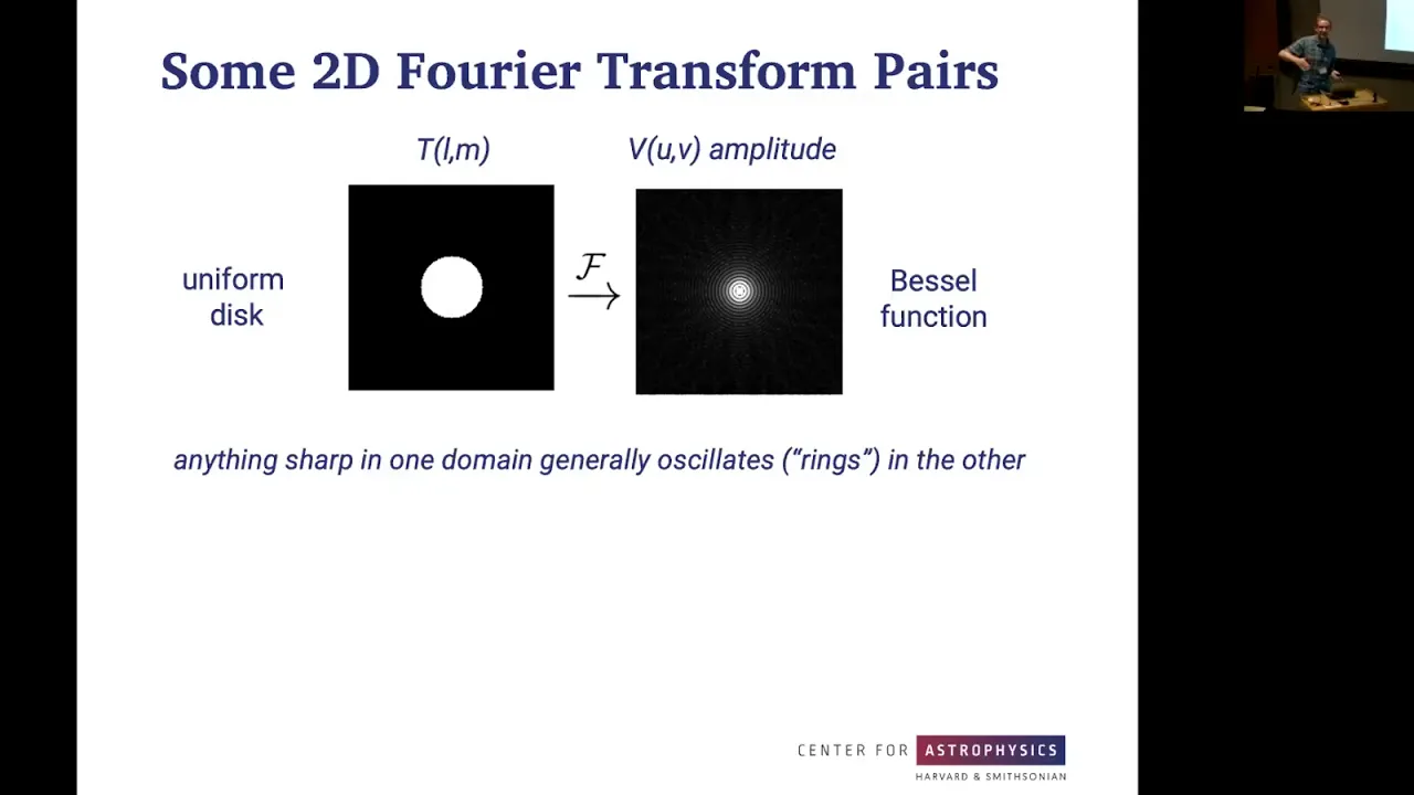
[00:00:03]well just as we as we've chosen U uh to be in this direction that also corresponds to the L Direction on the sky they point in the same direction um and W you'll recall is also the 1 minus L s- m^2 square root uh term in our source Direction uh the only term that we can't see here because we chose this Baseline so that had no V is the m Direction on the sky is is going to be uh into and out of the page here but if we look at this phase term this is really just the equation for a sine wave on the sky that has a Unity phase here that is one in the real component and zero in the imaginary component where U uh or L are zero and so because we've chosen the phase Center to be the center of our coordinates that is where L is zero right here this is the zero point uh then the response of this Baseline is going to look like a sine wave across the sky as we go in l and m so here I've drawn a somewhat homely sign wave on the sky that represents uh say the real component of the complex response of this interferometer on the sky in the L Direction and similarly if this Baseline had any projection along the V direction we would have some sine wave along the uh M Direction on the sky uh and so there's a sine wave and of course the imaginary component will be out of phase with this because one's a sign and one's a cosine uh when you do e to minus 2 pi I uh but this sine wave on the sky is something inherent to the response of this Baseline and it's called The Fringe pattern on the sky now I just said sine wave across the sky but there's something that is worth noting here um and that's the fact that l and m are not angles on the sky L is actually the sign of an angle in the East West Direction and M is the sign of an angle in the north south Direction and something else to note is that as u and v increase that is that your Baseline gets longer the frequency of the sine wave as a function of l and m increases so the longer your Baseline is the tighter this sine wave this Fringe pattern on the sky is going to be so I move these antennas twice as far away this this sign is sideway is going to go through uh twice as many uh periods across the sky as it does uh here and similarly if I move these antennas close together uh I'll have a much broader sine wave on the sky and this is all to say that the resolution the the size of features that you can pick up with the sign wave on the sky is dependent upon how far apart you've placed your antennas and this is why uh we often use an interferometer is because we can put two antennas of very large spacings and get much better resolution on the sky we can have a much tighter sine wave on the sky uh than we could if we had to fill in the entire area between these two antennas with metal so this picture right here is one way of understanding for uh just two antennas on the ground uh how they respond to the sky uh we could paint a sky on here choose an a uh primary beam and a I uh the distribution of of flux density on the sky and uh by painting this this uh Fringe pattern on the sky we can say what the response of this Baseline is going to be at any given UV and w now what I'm going to do is actually just give a intuitive understanding of what's going on here that gets away from choosing any particular two pairs of antennas instead kind of holistically looks at the process of sampling a sky with many antennas uh all together in Array and talking about the response of that entire array I'm going to clear out a little space here and I'm going to to erase up to this equation that we have up here where I've bracketed the W term and so we recall that this is still a 4A transform we've just neglected one of the terms here and uh we'll we'll visit that term later but it's multiplied by the rest of what we do so worst case scenario we have a 4A transform here and because we have a product inside of the 4A transform that's the same as a convolution outside it so uh the fact that I'm erasing this and ignoring this term for now doesn't change the fact that this is a 4A transform even if there's a function convolving it that we haven't discussed yet um also now that I've erased and gotten some room going to remind you that this uh bracketed term here uh was the perceived Sky um and I'm going to talk about everything in terms of the perceived sky right now because uh it's just a little too much detail to track primary beam responses through all of this so I'll begin by drawing a dotted line down the middle of the page here and on one side here I'm going to draw big two-dimensional uh picture of the sky so we'll call this the sky um and I'm going to draw a Big Dipper on here for fun and we know that if this is the sky and we'll actually just say that this is the perceived Sky then the for a transform of that which goes across to the other side of the page transforms our l and m coordinates on the sky to u and v coordinates uh so the 4 Transformer of the sky has coordinates of u and v uh creatively it's called the UV plane and that UV plane is what an interferometer with coordinates of u and v and we ignored the W component so u and v are Baseline length this is what uh a baseline in an array a pair of antennas samples is the UV plane and I'm going to draw this so that U of z v of0 is right here in the middle so I've written that this is a UV plane here but I should clarify that this is the true UV plane uh if we had a whole bunch of antennas covering an entire field and we covered every every piece of that field we might be able to sample every unv and recover the true UV plane but in practice that just doesn't happen so let's suppose for a minute that we only have three antennas in a field I'll label them a b c now if we want to keep track of all the baselines that we have there I'm going to draw the interferometric sampling of this array so this is what the sampling of the UV plane is going to look like uh so if we draw a vector from A to B that points to right up here that's one of the samples we'll get a to c will Point straight to the left uh and B to C will Point down um and uh I will also put a little circle here in the middle to show that um a AA is actually a baseline an antenna with itself and that samples the center of the UV plane at U v0 and say and BB also samples there and CC does as well uh so we other than these which are called autocorrelations uh we have three uh samples of the UV plane here but I chose to measure a to B but in fact B to a is a perfectly valid sample as well so why did I draw a DOT up here and not down here uh for a vector pointing the opposite direction and the fact is that I actually can I do get that sample um but it's not an independent piece of information so maybe I should color this a different color I'm going to color it Orange that the orange samples here are reflections of the Baseline so if this was AB then ba is over here but they don't have independent information and the reason is that the sky here is real valued uh we don't get complex waves from the sky we get real valued electric waves uh electric fields that come in and the uh the consequence of that for knowing that we have a real valued sky is that uh for any uh coordinate any spatial frequency which is what u and v are for any spatial frequency out here uh the corresponding negative frequency the value that you measure in it has to be the complex conjugate of what you measure at a positive frequency that's just what happens when you take for a transforms of real valued signals so if I measured V over here then it's absolutely true for a real value sky that I would have to measure V conjugate over here V Star so for any Baseline that I measure V I can put two points on this UV plane one at the u and v coordinates of the Baseline in One Direction and one at the minus U and minus V coordinates uh in the other direction uh but the catch is I have to conjugate my visibility if I were going to put it there so a baseline at minus U minus V which is just pairing your antennas backwards will have a conjugate value coming out of your correlator then if you uh correlate a with B so B with a and a with B come out with a different conjugation out of your correlator depending on the order that you correlate them but uh for whatever you get out of the correlator you can always put the other uh sample down now one last little cute thing here is uh just as a bit of an aside that we went from the distribution of antennas on a field here A B and C to the UV sampling pattern now it turns out you if you want to calculate this fast uh faster than what we just did which was pairing every antenna with every other antenna you could just make a little Matrix here put down your antenna positions as dots in that Matrix and then convolve that Matrix with itself and what that does is it slides A and B and C uh by a copy of itself in any place where a and b or a and C or B and C line up it's going to put a dot at that separation so uh interestingly the UV sampling of an array is just the convolution of the distribution of antennas in a field with itself so now we have our true UV plane which is a for a transform of the perceived sky and we have uh our UV sampling pattern which reflects that for any array that we have we don't get all of the information in the UV plane so those combined suggest that what we truly measure here is a sampled UV plane where we've put in at each u and v coordinate and at each minus U and minus V coordinate the visibility that we measured uh on our ineter out of our correlator and everywhere else uh we've just put zero because we have no information about any unv of the true UV plane that we haven't sampled with our the inherent UV sampling of our array so we have incomplete information but we might as well just go ahead and do the 4A transform of our sampled UV plane and see what we get and what we're going to get is something that looks like our true Sky you'll see something that looks like the Big Dipper here but around each point here uh we're going to have little things coming out and it's going to look a little grungy these are called side loes so this is a a grung it's a dirty view of the sky and in fact this is often called the Dirty image the dirty image is the direct inverse transform of the sampled UV plane so why do we not get back our perfect Sky well we lost information what we did is we took the true UV plane which is what you can for a transform to get your Sky back and we multiplied it by our UV sampling pad