Adaptive Optics: Physics, Engineering & Control

Learning Goal: Mastering the engineering and physics of adaptive optics (AO) systems in modern ground-based observatories. This includes mathematical modeling of atmospheric turbulence, high-speed wavefront sensing, the physics of laser guide star generation, the mechanical engineering of deformable mirrors, and real-time control loop execution.

Prerequisites

To get the most out of this curriculum, you should have a solid foundation in:

• Physics: Electromagnetism, classical wave mechanics, and physical optics (diffraction, interference).
• Mathematics: Multi-variable calculus, Fourier analysis (Fourier series and transforms), and linear algebra (specifically matrix operations, eigenvalue decomposition, and singular value decomposition).
• Programming: Basic proficiency in Python or MATLAB for numerical simulation.

Estimated Total Study Time

35 Hours (including video lectures, recommended mathematical derivations, and hands-on simulation practice).

---

Module 1: Foundations of Wave Optics and Wavefronts

This module establishes the wave theory framework necessary to understand light propagation. You will transition from geometric ray tracing to wave optics, focusing on how phase perturbations scale, how wavefronts are defined mathematically, and how optical systems are fundamentally constrained by the diffraction limit.

• Why this video: This video bridges theory and implementation by showing how to numerically simulate optical diffraction patterns using Python. It teaches you how to map physical apertures and wavefront aberrations to the far-field diffraction pattern (the Point Spread Function, or PSF) using Fast Fourier Transforms (FFTs), which is the computational backbone of wave optics modeling.

---

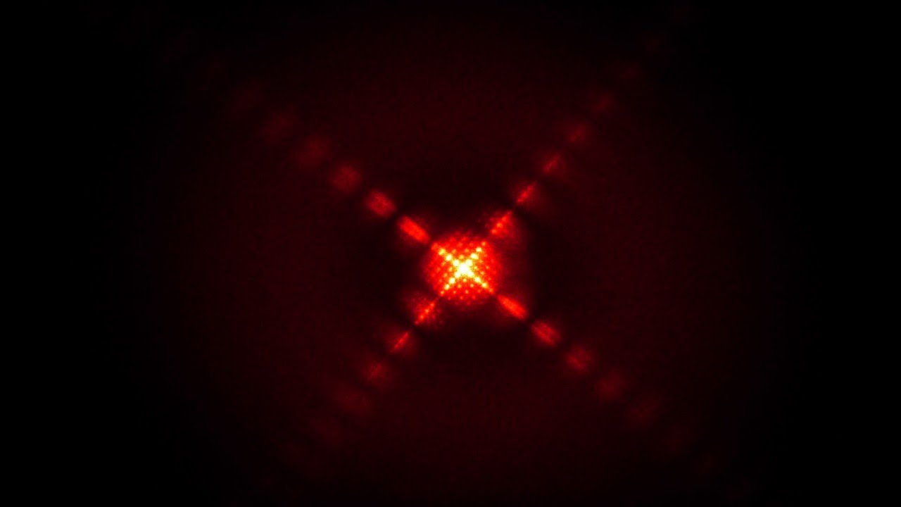
• Why this video: Understanding how optical components manipulate wavefronts in space is critical. This video provides an intuitive and physical explanation of the 4F correlator, showing how a simple lens physically performs a Fourier transform on a wavefront, mapping spatial coordinates to spatial frequencies.

---

• Why this video: A rigorous academic definition of a wavefront is essential before manipulating it. This brief lecture segment from MIT defines wavefronts as surfaces of constant phase in 1D, 2D, and 3D space, which is the exact mathematical entity that adaptive optics systems aim to measure and correct.

---

Knowledge Checkpoint

• Define a wavefront mathematically as a function of spatial coordinates $(x, y, z)$ and time $t$.
• Explain how a positive thin lens converts a planar wavefront into a converging spherical wavefront, and how this relates to the optical Fourier transform.
• Explain the diffraction limit of a circular aperture telescope using the Airy disk formula ($\theta \approx 1.22 \lambda / D$).
• Write a basic Python script using numpy.fft to simulate the diffraction pattern of a square or circular aperture.

---

Module 2: Statistical Optics and Atmospheric Turbulence

To correct the effects of Earth's atmosphere, you must model it mathematically. This module covers Kolmogorov's model of turbulence, showing how index of refraction fluctuations warp flat wavefronts. You will learn about key statistical parameters, including Fried's parameter ($r_0$), astronomical seeing, and the Greenwood frequency ($f_G$).

⚠️ Pedagogical Note on Video Coverage: The public video pool contains fewer rigorous engineering lectures on Kolmogorov turbulence statistics. To supplement these videos, we highly recommend researching the mathematical derivations of the phase structure function $D_\phi(r) = 6.88 (r/r_0)^{5/3}$ and the Greenwood frequency $f_G \propto v/r_0$. Use the search query: "Kolmogorov turbulence theory optical propagation lecture".

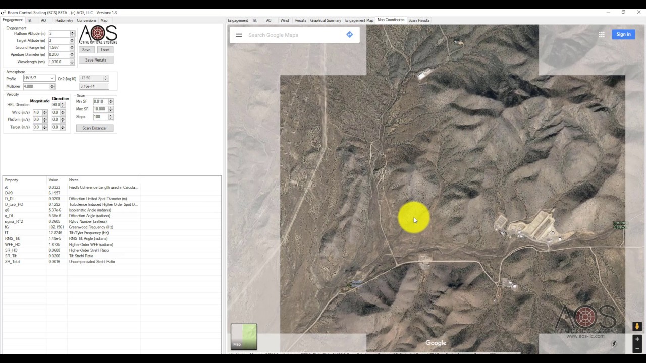
• Why this video: This highly technical tutorial steps through the engineering software tools used to estimate atmospheric propagation characteristics. It demonstrates how physical parameters like Fried's coherence length ($r_0$) scale with wavelength and zenith angle, and how these parameters govern system performance.

---

• Why this video: This lecture segment provides the academic physics context for Kolmogorov turbulence. It discusses the scaling of spectral energy density within the inertial range (scaling as $k^{-5/3}$), which is the exact statistical model used to characterize index of refraction fluctuations in Earth's atmosphere.

---

• Why this video: A concise professional summary explaining that optical turbulence arises from micro-thermal variations in the air, which in turn cause rapid variations in the local refractive index.

---

Knowledge Checkpoint

• Explain the physical mechanism of Kolmogorov turbulence, from the outer scale ($L_0$) where energy is injected, through the inertial range, down to the inner scale ($l_0$) where energy dissipates.
• Define Fried's parameter ($r_0$) physically. What does it mean when a telescope's aperture diameter $D$ is much larger than $r_0$?
• State the relationship between Fried's parameter and the wavelength of light ($r_0 \propto \lambda^{6/5}$). Why is adaptive optics easier to implement in the infrared than in the visible spectrum?
• Define the Greenwood frequency ($f_G$) and explain how it determines the required correction rate (bandwidth) of an adaptive optics real-time control system.

---

Module 3: Wavefront Sensing Technologies

A wavefront sensor (WFS) measures phase errors in real time by converting phase variations into measurable intensity variations. This module examines the optical design and mathematics of the two dominant wavefront sensors: the Shack-Hartmann sensor and the Pyramid wavefront sensor.

• Why this video: This university workshop lecture by Dr. Becky Jensen-Clem provides a rigorous review of wavefront sensing technologies in astronomy. It covers the mechanics of Shack-Hartmann sensors, describing how lenslet arrays sample the wavefront and measure local phase gradients ($\nabla \phi$).

---

• Why this video: This video highlights the advanced physics comparison between the classical Shack-Hartmann design and the modern Pyramid Wavefront Sensor. It demonstrates how the Pyramid sensor offers increased sensitivity, especially for low-order aberrations (like tip-tilt), allowing observatories to use fainter guide stars.

---

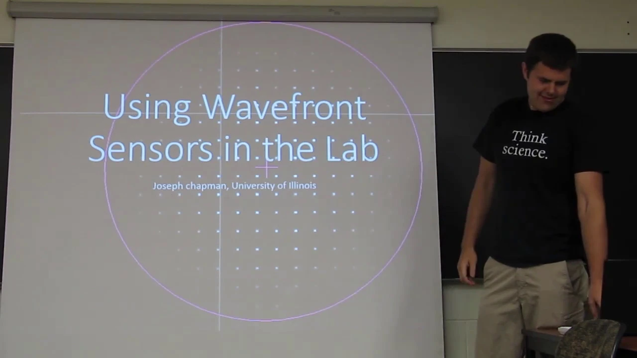
• Why this video: This experimental demonstration shows how a Shack-Hartmann sensor uses a microlens array to split an incoming wavefront into a grid of focal spots. You can see how wavefront distortions translate directly into focal spot displacements on a CCD/CMOS sensor.

---

Knowledge Checkpoint

• Derive the relationship between the local wavefront gradient (slope) over a subaperture and the physical displacement $(\Delta x, \Delta y)$ of the focal spot in a Shack-Hartmann sensor.
• Describe the optical design of a Pyramid wavefront sensor, including the four-faceted glass pyramid and the four resulting pupil images on the detector.
• Explain why the Pyramid WFS has a higher sensitivity limit (or lower noise propagation) compared to the Shack-Hartmann WFS when correcting low-order aberrations.
• What is the "linearity range" of a wavefront sensor, and why is sensor modulation used in Pyramid sensors to balance linearity and sensitivity?

---

Module 4: Laser Guide Star (LGS) Engineering

Natural guide stars bright enough for wavefront sensing are rarely located near the astronomical targets of interest. This module covers the physics of generating artificial guide stars using sodium resonance and Rayleigh scattering lasers, while examining the geometric limitations of these systems.

⚠️ Pedagogical Note on Video Coverage: The video pool contains fewer in-depth engineering breakdowns of the "cone effect" (focal anisoplanatism). To master this key limitation, we recommend studying how a finite-altitude LGS creates unsampled atmospheric volumes compared to a natural guide star at infinity. Use the search query: "Focal anisoplanatism cone effect adaptive optics".

• Why this video: Professor Niranjan Thatte explains the core physics of the "cone effect" (focal anisoplanatism). Because laser guide stars are generated at a finite altitude (~90 km for sodium), the backscattered light traces a cone rather than a cylinder, leaving the upper-altitude atmospheric turbulence near the edges of the telescope aperture unsampled.

---

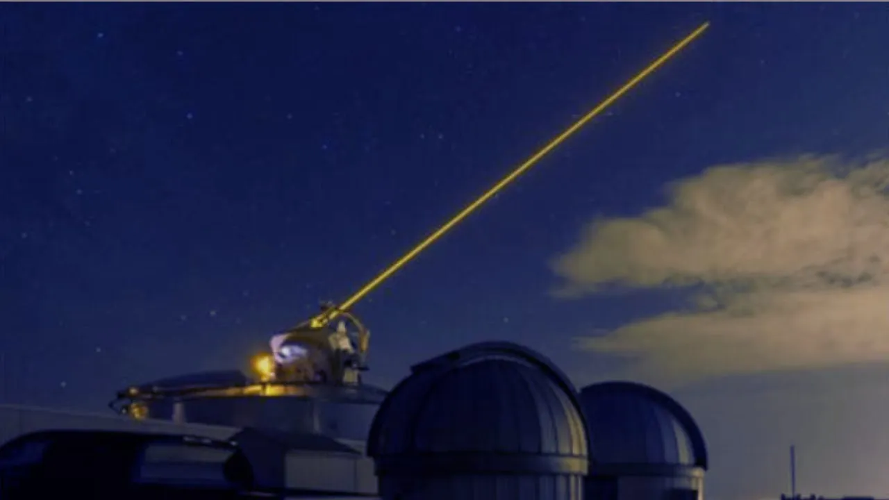
• Why this video: Dr. William Happer, one of the key physicists behind the development of the technology, explains the atomic physics of exciting the mesospheric sodium layer (at an altitude of ~90-100 km). He describes how a laser tuned to the $D_2$ transition line of sodium (589 nm) makes the atoms fluoresce, creating an artificial star.

---

• Why this video: Provides the historical and military-scientific context of the declassification of laser guide star technology. It highlights how the defense advisory group (JASON) solved the high-altitude atmospheric fading problem by shifting from low-altitude Rayleigh scattering to high-altitude sodium layer resonance excitation.

---

Knowledge Checkpoint

• Explain the difference in physical scattering mechanisms and operating altitudes between a Rayleigh LGS (scattering off air molecules up to ~20 km) and a Sodium LGS (resonance excitation of sodium atoms at ~90 km).
• Define "focal anisoplanatism" (the cone effect) mathematically and explain why its severity scales with telescope diameter $D$.
• Explain why a single laser guide star cannot measure "tip-tilt" (positional jitter) of the wavefront, and describe how astronomers solve this using a faint natural star as a secondary reference.
• Describe the optical design solution of "Laser Guide Star Asterisms" (using multiple lasers in Laser Tomography AO or Multi-Conjugate AO) to overcome the cone effect.

---

Module 5: Deformable Mirrors & Wavefront Correction

Once the wavefront error is measured, it must be physically corrected. This module covers the mechanical and material engineering of Deformable Mirrors (DMs), focusing on thin-shell membranes, piezoelectric actuators, and Micro-Electro-Mechanical Systems (MEMS).

• Why this video: An exceptional engineering deep dive into the physical construction of a deformable mirror. The video shows how a thin reflective face sheet is mounted onto a matrix of electromagnetic actuators, explaining key concepts like actuator coupling, stroke limit, and structural mechanical limits.

---

• Why this video: Professor Thomas Bifano, a leading researcher in MEMS deformable mirrors, explains how silicon micro-fabrication enables high-actuator-density DMs at a fraction of the cost and size of traditional piezo mirrors. He details the electromechanical modeling, stroke limits, and sub-nanometer resolution capabilities of MEMS-based systems.

---

• Why this video: This video links the high-precision shaping of deformable mirrors with advanced coronagraphy for direct imaging of exoplanets. It shows how DMs are used not just to correct atmospheric turbulence, but also to create "dark holes" in the stellar diffraction pattern by canceling out tiny quasi-static optical aberrations.

---

Knowledge Checkpoint

• Explain the concept of "actuator stroke" and distinguish between the inter-actuator stroke and the global stroke of a deformable mirror.
• Describe how an actuator's "influence function" defines the localized mechanical deformation of the mirror's face sheet when a single actuator is poked.
• Compare piezoelectric, electromagnetic, and electrostatic (MEMS) actuator technologies in terms of actuator density, response speed, and maximum physical stroke.
• Explain the mechanical danger of "actuator coupling" and how mirror designs minimize localized shear stress on the thin glass face sheet.

---

Module 6: Real-Time Control Systems and Algorithms

Adaptive optics systems must run feedback loops at kilohertz frequencies to stay ahead of changing atmospheric turbulence. This module covers the mathematical framework of wavefront reconstruction (using interaction and reconstruction matrices) and the high-speed hardware required to execute these calculations.

⚠️ Pedagogical Note on Video Coverage: The video pool contains general PID control lectures, but has limited coverage of the unique linear algebra required for multi-input multi-output (MIMO) wavefront reconstruction. To master this, you should study how Singular Value Decomposition (SVD) is used to invert the non-square "Interaction Matrix" ($G$) to produce the "Reconstruction Matrix" ($R = G^\dagger$). Use the search query: "Wavefront reconstruction matrix interaction control loop adaptive optics".

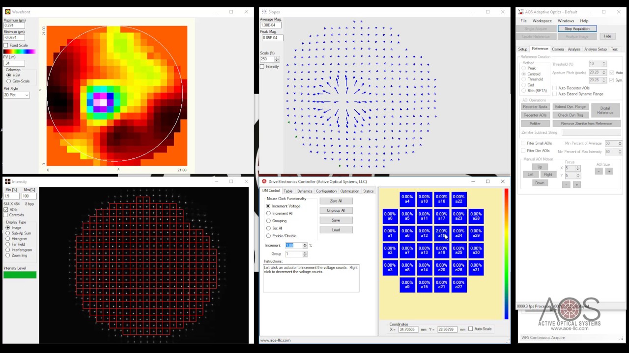
• Why this video: This software demo provides a practical look at how an AO system calibrates itself. It demonstrates "poking" individual actuators to record their influence functions on the wavefront sensor, which is the exact physical procedure used to build the Interaction Matrix. It then shows the Singular Value Decomposition (SVD) calculation used to generate the system's control matrix.

---

• Why this video: This video demonstrates how to run a closed-loop adaptive optics simulation in MATLAB using the ACE toolbox. It visualizes the active feedback loop, showing how slope measurements from the WFS are converted into actuator commands to minimize residual wavefront errors in real time.

---

• Why this video: Modern AO systems rely on Field-Programmable Gate Arrays (FPGAs) or high-performance GPUs to process calculations with sub-millisecond latency. This industry discussion highlights how FPGAs enable adaptive, parallel hardware acceleration, which is critical for executing high-speed matrix-vector multiplications.

---

Knowledge Checkpoint

• Write down the matrix equation relating the vector of wavefront sensor slope measurements ($s$) to the vector of actuator commands ($a$) via the Interaction Matrix ($G$): $s = Ga$.
• Explain how Singular Value Decomposition (SVD) is used to calculate the pseudo-inverse $G^\dagger$ (the Reconstruction Matrix $R$), and how you handle poorly-conditioned eigenvalues (null modes like piston).
• Draw a block diagram of a classic closed-loop adaptive optics system showing the wavefront sensor, the Real-Time Controller (RTC), the Deformable Mirror (DM), and the science camera.
• Define "latency" (or delay time) in an AO control loop and explain how processing delays affect the overall correction performance (Strehl ratio) as wind speed increases.

---

Course Map

This flowchart shows the dependency path and recommended study order for mastering Adaptive Optics:

---

Key People Index

• Dr. William Happer (Princeton University / JASON Group): A pioneer in atomic physics who co-conceived the sodium laser guide star. He proposed tuning laser lines to the $D_2$ resonance line of mesospheric sodium atoms to create high-altitude artificial reference stars.
• Dr. Andrea Ghez (UCLA): Awarded the 2020 Nobel Prize in Physics for her discovery of the supermassive black hole (Sagittarius A*) at the center of our galaxy, a milestone discovery made possible by using high-resolution adaptive optics on the Keck telescopes to track stellar orbits.
• Professor Thomas G. Bifano (Boston University): A key pioneer in the mechanical engineering and microfabrication of MEMS-based deformable mirrors. His research enabled ultra-precise, high-density wavefront correction systems.
• Dr. Becky Jensen-Clem (UC Santa Cruz): An astrophysicist and professor specializing in the design, testing, and implementation of extreme adaptive optics systems for exoplanet direct imaging.

---

Final Self-Assessment

To verify your mastery of the physics, engineering, and control mechanics of adaptive optics, you should be able to confidently check off every item in this comprehensive self-assessment:

• Explain how a wavefront is defined as a surface of constant phase, and prove mathematically how a 2D Fourier transform relates a perturbed pupil-plane wavefront to its far-field Point Spread Function (PSF).
• Calculate the atmospheric coherence length ($r_0$) and the Greenwood frequency ($f_G$) given a profile of the refractive index structure constant $C_n^2(z)$ and wind speed $v(z)$.
• Formulate the mathematical equations that convert Shack-Hartmann centroid offsets $(\Delta x, \Delta y)$ to local phase gradients, and describe how these gradients map to the interaction matrix $G$.
• Compare the optomechanical designs of Shack-Hartmann and Pyramid wavefront sensors, and explain why the Pyramid sensor has superior sensitivity at low spatial frequencies.
• Detail the physical process of generating a sodium laser guide star, including the laser wavelength required ($589\text{ nm}$), the physical layer altitude ($\sim 90\text{--}100\text{ km}$), and the atomic transitions involved.
• Describe the "cone effect" (focal anisoplanatism) mathematically, and explain why it requires multi-laser tomographic systems on extremely large telescopes (ELTs).
• Diagram the mechanical cross-section of a piezo-actuator and a MEMS-actuator deformable mirror, comparing their stroke limits, response times, and actuator spacing limits.
• Perform a Singular Value Decomposition (SVD) on a toy $3 \times 2$ interaction matrix, identify any uncorrectable null modes (like piston), and write down the corresponding reconstruction matrix.
• Define the Strehl Ratio ($S$) and explain how it degrades in relation to the residual wavefront phase variance $\sigma^2$ using the Maréchal approximation ($S \approx e^{-\sigma^2}$).
• Design a block-diagram architecture for a $1\text{ kHz}$ real-time control system, specifying the roles of the WFS detector, FPGA/GPU matrix-vector multiplier, and the digital-to-analog converters (DACs) driving the deformable mirror.