DIY Deformable Mirror Design for Adaptive Optics

[00:00:03]Hi everyone, It’s been a while since I made my last video. That’s because I was busy with doing  other stuff like making telescope mirrors. Most things were actually quite unexciting apart from  one exception: my visit to the ZERODUR production facility of Schott in Mainz, Germany a few weeks  ago. The people at Schott invited me to take a look at some of their manufacturing processes,  an opportunity that of course I couldn’t resist.

[00:00:28]I got to see how blocks of hot glass weighing  over 2 ton were quickly cooled down to below the nucleation temperature. And let me tell  you: the amount of heat that these release during cooling is really mind boggling, it’s  enough to turn huge production halls into cozy infrared saunas. I also got a tour around the CNC  manufacturing facilities which can process parts up 6m in diameter with very high-precision. And  apart from polishing to optical specification, they basically do everything in house. Now of course, to make these parts to spec, you also need to be able to measure them and  to do that, you can’t use a simple caliper. So instead they have a rather substantial coordinate  measurement machine that has an accuracy of 1.5 microns over several meters of distance. To  achieve this, the hall where the instrument is located is temperature controlled to 0.1  degree C. That is what these air inlets are for. All in all the visit was pretty impressive.  So I want to thank the people at Schott for this opportunity. And just to be clear: this  video is not in any way sponsored by Schott, I just wanted to show you this. Anyway let’s not get too much distracted from the main subject of this video, which  is making adaptive optics. In particular: making a deformable mirror. Now, deformable  mirrors are for example used in large earth based telescopes to improve image quality.  The reason is that the image resolution of a traditional earth-based telescope is limited by  atmospheric turbulence. Turbulence is basically the flowing and mixing of air that has different  temperature and humidity levels. Due to this, the atmosphere contains small but rapidly  changing variations in refractive index and this causes small disturbances in the wavefront  of light when passing the atmosphere. Which in turn cause un-sharpness in the images recorded.  And the amazing thing is that adaptive optics can correct for the effects of turbulence and recreate  the original sharpness. So how does this work?

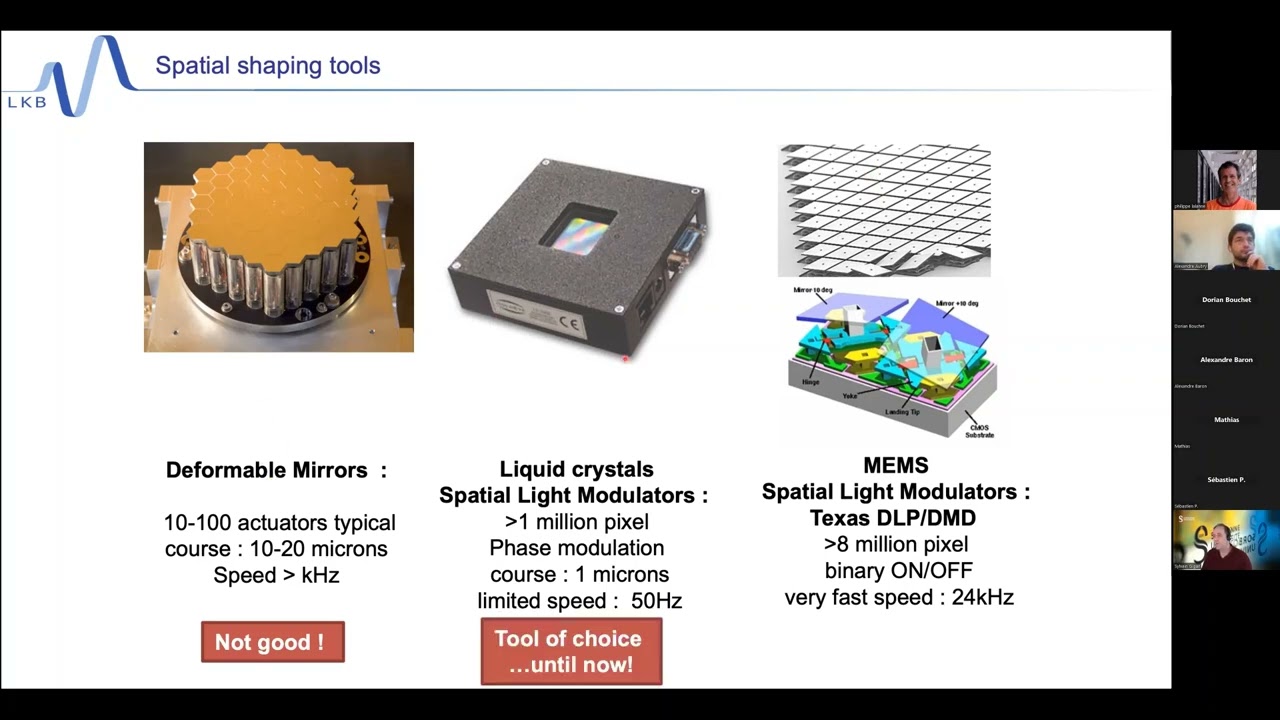
[00:02:34]Well, a commonly used method is creating an  artificial star with known properties by using a beam of light from a sodium laser. This artificial  star is created in In the mesosphere, which is about 90km above ground level. The mesosphere  is also rich in sodium which originates from asteroids burning up in the higher atmosphere.  And the laser can excite these molecules and force them to reemit light at a very distinct  wavelength. And this creates an artificial star that can be observed with the telescope. Now in  a traditional telescope, all optical surfaces are fixed and are manufactured to a very accurate  shape. This shape would result in a good image with no wavefront distortion being present in  the light. However if the wavefront is distorted, the light is actually ending up in the wrong  place on the sensor. So to solve this problem, one of the mirrors like for example the secondary,  is replaced with one that has a variable surface shape. So this is illustrated here where mirror  surface itself is on a relatively thin sheet of curved glass. This sheet is generally only a  few mms thick and is attached to a bunch of linear actuators. And what this mirror can do is  dynamically change its surface shape such that it exactly counteracts the wavefront errors present  in the incoming light And if you do that very quickly and with high accuracy, you can keep the  telescope “focused” regardless of turbulence.

[00:04:00]But of course, we need to know what the shape  of this deformable mirror must be to do this.

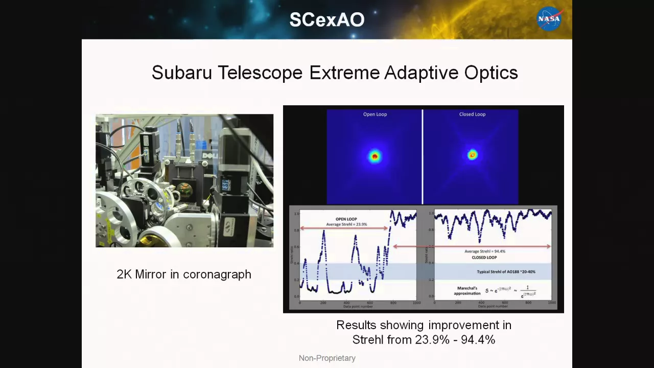
[00:04:05]And this is where the artificial star comes  in. It can easily be isolated from the rest of the image by optical filtering at its emission  wavelength. The stars’ image is then projected on a wavefront sensor that can measure the shape  of the wavefront which is then analysed. And then a complex matrix calculation is done  to establish the desired position of each individual actuator and change the shape of  the deformable mirror surface accordingly.

[00:04:31]Now, the effects of turbulence typically occur  on the millisecond time scale. So within a timeframe of approximately a millisecond, you  have to measure the wavefront, then calculate the desired change in surface shape to correct  for the error and then apply these corrections to the mirror surface. For this reason, the  adaptive mirror surface itself must be thin and lightweight. And that is why adaptive optics are  generally not implemented in the large and heavy mirrors like the primary, because that would  make fast changes in shape very difficult.

[00:05:04]Here are a two examples of adaptive mirrors  that are actually used in telescopes: this is the adaptive secondary that was  made by TNO the Netherlands for the IRTF, an infrared telescope of the University of  Hawaii. Fun fact: I actually made a small contribution to this mirror by cutting and  polishing the face sheet. It was then send to TNO where it received an aspherical shape  correction and was then coated. And these blue cylinders containt the actuators that can  pull and push the surface into the desired shape. Here is another example from the Multiple  Mirror Telescope in Arizona. This one has 336 actuators to press the surface into the correct  shape. And maybe now you wonder why so many?

[00:05:48]Well the effects of turbulence not only occur  on a typical time scale of milliseconds, but also on a typical dimensional scale, described  by the Fried parameter which refers to the maximum aperture size that leads to an undistorted image.  And the typical value for the Fried parameter is around 100-200mm for normal atmospheric conditions  and maybe 300-400 for a very quiet atmosphere.

[00:06:13]So if you have a small telescope smaller than  the typical Fried value, the turbulence mainly changes the angle slightly at which we observe  an object. However, with very large telescope, the total wavefront error over the telescope  aperture is the result of multiple turbulent cells and this in turn results in a wavefront that  contains fairly complex deformations within the total aperture. So to correct for this you need  sub-aperture or local corrections of the wavefront in the optic. Now the current MMTs primary has a  diameter of 6.5m, which explains why you need so many actuators to correct for wavefront errors. In this image I sort of summarized what kind of aberrations you can expect based on telescope  aperture: if you have a telescope with a diameter that is smaller than the Fried parameter,  you basically only have to correct for small angular variations. And this can be done by the  introduction of what we call prismatic corrections like tip and tilt. Basically, this is a form of  fast image stabilization. Now if we look at larger diameter telescopes, the total wavefront error can  only be corrected by a combination of more complex aberration types. So the larger the telescope  aperture, the more complex the corrections need to be to “undistort” the wavefront. Okay, let’s do something practical with this concept. Now you can imagine that I’m not going  to make a fancy multi-million dollar adaptive optical system with all the electronics.  Instead I want to focus here on making the deformable mirror part. So just the face  sheet with some actuation. And not one with hundreds of them but a limited number. Lets first discuss the design I had in mind. I want to start out with a relatively  rigid support plate as the mechanical basis.

[00:08:03]On the surface here I indicated the positions of  a total of 25 actuators, which will be glued to this back plate. If we zoom in on an individual  actuator, we see that it consist of a central pillar made of a flexible material like for  example a silicon rubber. The pillar itself is inside a small reel or bobbin that consist of  2 parts to simplify the manufacturing. And this can be used to wind a copper coil on, so this  will hold the electromagnet. And we can run a variable current through the coil to attract  or repel the magnet that is glued on top of the silicon pillar. So that is basically the whole  actuator construction, pretty simple. The only thing still missing here is the face sheet, which  represents the deformable mirror. This is just a sheet of glass glued to the magnets. Since we are  not going to put this thing into a telescope and it’s just a prove of principle, we can settle  for a flat piece of glass for now. This also make manufacture and measuring deformations a  lot easier then when using a curved surface.

[00:09:06]Here is a cross section of a finished actuator.  Depending on the polarity and the current through the coil, a variable attractive or repulsive force  can be exerted on the magnet and therefore on the face sheet. And so, in theory we have a very  simple and direct way to deform the shape of the face sheet surface. Of course, the extend of  the deformation would be very dependent on the thickness of the face sheet and the forces that  can be exerted on the magnets. At this point, we do not have a good idea about what kind of forces  will act on the face sheet and what this means for the thickness of the face sheet. It probably has  to be quite thin because the actuators are small and can likely not exert large forces anyway. This  means that for example a 4mm Robax sheet will be way too thick because you need several newtons  of force to change the shape significantly.

[00:09:58]So what I’ll do is start out with a face sheet cut  from an old quartz photomask, which is 2.3mm thick and is pretty flexible on the micron scale.  But if that is not sufficiently thin enough, I’ve got another option: Maybe you remember that  at the end of the last video I had received a mystery package from Japan. This package was very  kindly sent to me by the people at Nippon Electric Glass Company. Don’t be fooled by the dimension of  the package: it just contains 2 relatively small glass plates with a thickness of only 1.6 and  1.3mm respectively. But this is no ordinary glass.

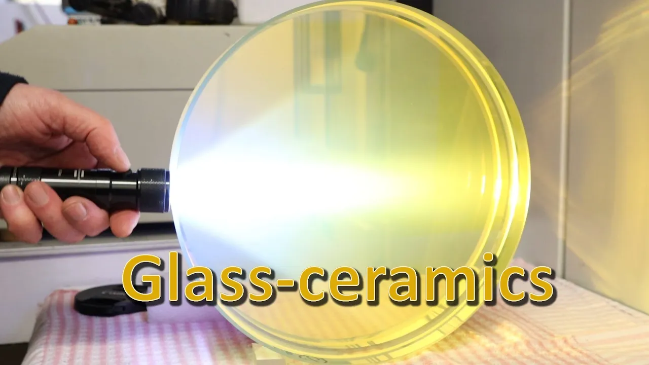
[00:10:35]This is a zero-expansion glass-ceramic that comes  in thin sheets and which is appropriately named ZERO. If you look at the thermal expansion of  this material as a function of temperature, you can see that it hardly contracts or expands. Even  over a temperature range of -40 to +80 degrees C, it expands less than 2 micron per meter of length,  which translates to 0.016 ppm/per degree Celsius, which is pretty impressive. Now it was not  my initial intention to use this material to make a face sheet from. But as hopefully will  become clear there might be some advantages to using zero thermal expansion in the current  application because of heat development. Anyway, these sheets are certainly quite a it more  flexible because they are so thin. Unfortunately, they are also not very flat, which might  be a bit of a problem. So let’s just start with using the quartz plate and  if that doesn’t work try these, because making them flat will be quite  a challenge. Okay, so let’s do this.

[00:13:17][Music] So this is the complete device. Now if I connect  the central 9 actuator coils to a high-frequency square wave, I think it is a little over 2  KHz, you can clearly hear this annoying tone.

[00:14:39]So the face sheet is moving up and down with this  frequency and starts acting like a speaker cone.

[00:14:45]So it seems that in principle we can move  the face sheet up and down pretty fast.

[00:14:50]Let me quickly discuss the choice for the  copper wire thickness in the actuator coils, because this is actually kind of an interesting  aspect. You probably know that a current running through a wire creates a magnetic field. And  if you wind this into a coil, the magnetic field in the coil is proportional to both the  number of turns and the current running through the wire. Now, as for the magnetic attraction or  magneto-motive force on a magnet: this property is not proportional to the magnetic field itself but  to the gradient in the magnetic field. That said, if we have a field with a constant shape with a  magnet held in a more or less static position, is to be expected that the force acting on the  magnet will be proportional to the number of turns times the current running through the wire. Now it is tempting to think that because of this, we want a lot of turns. Because with the same  current we can exert a higher force on the magnet.

[00:15:43]And even though this is in principle true, we are  actually not interested in the current running through the coil; we are interested in the amount  of power dissipated by the coil. Because that determines how hot these will get when we will run  a specific current through them. For a resistive wire, the power dissipated is the current squared  times the resistance. So what is the optimum value for the number of turns, given that we have a  limited volume available in the bobbin and we have a maximum value for the dissipated power that is  allowed? Well, the answer is kind of surprising: Let’s start out from the assumption that the  magneto-motive force is proportional to the number of turns times the current. The number of  turns that we can create in the coil is the volume of the coil (Vc), divided by the cross section  area of the wire (Aw) times the mean length of a single turn (Lm). Pretty straight forward:  basically this the total coil volume available divided by the mean volume of a single the wire  turn. Now, the current and the wire resistance are what makes a coil dissipate power and if we  assume certain maximum power dissipation level, the corresponding current is equal to the  square root of this maximum power divided by the internal resistance of the coil. On the  other hand: the resistance of the total wire can be written as the conductivity (in this case of  copper) times the volume of the coil divided by the wire cross section area squared. I’m not going to write this all out, but if you combine these, you can arrive at a  formula that shows how the force on the magnet is proportional to the length of a single turn,  the power dissipated, the total coil volume and the resistivity of the conductor. And what is  surprising here is that the number of turns (n) is nowhere to be found in this formula. It  is just about coil dimensions, conductivity and the amount of power you are dissipating. So in  essence, it does not matter whether you use 6, 20 or 80 turns. When power dissipation is the  parameter you steer on, any of these numbers will result in approximately the same force on  the magnet at a set power dissipation level. Of course there are a few practical details here:  a very thin wire might have a relatively thick isolator mantle so that would actually not  help because it would reduce the amount of copper you can get into the coil volume and  increase resistance. Also it would reduce the thermal conductivity of coil itself. But in the  end a choice for a particular wire thickness is about which is most appropriate for you driver.  Apart from that, it does not really matter.

[00:18:22]Anyway, with the choice of the number of turns  and wire diameter being more or less irrelevant, I did a few tests and chose 0.22mm wire. Mainly  because it allowed me to make coils that had a DC resistance of 1 ohm which is convenient: to run it  at 1 Amp you need 1V and it produces 1 W of heat.

[00:18:42]And it turns out that the force that is generated  is around 0.1N with the 6mm diameter magnets that I used. I must admit that this is less than  I expected, but let’s try to work with it.

[00:18:54]Okay, let’s first try to measure the face  plate as is, in the interferometer without any currents running through the coils. And for this  measurement we don’t want the top surface to have a highly reflective mirror coating because the  interferometer compares the surface with a flat that has 4% reflection, the same as an uncoated  glass interface. So here you see the setup with the deformable mirror, the interferometer with  the reference flat on this side. I have opened the interferometer up to expose the camera.  This camera is connected to the laptop PC.

[00:19:26]Those of you that are familiar with DFTfringe  will have noticed that I’m using a different type of software here. So, while I was considering  making this video I was contacted by Jaco Verster, a researcher from South Africa who was developing  near-real-time interferometry software. He asked if I was interested in testing it and give  some feedback. Which of course I was because I thought this project would be the perfect  test case for that. The software is called Wavefront Pro and you will find more information  in the description of this video. The reason for using it here is that it performs a wavefront  measurement from an interferogram every second or so. And this feature allows for measuring  wavefront shape almost in real time. This allows us to immediately see how much the face  sheet deforms when we activate the actuators.

[00:20:18]I think it is good to point out that Wavefront  Pro since it has been developed recently does not have same functionality as DFTfringe. Its  not suited for evaluating a-spherics and does not calculate wavefronts with the same level of  detail. But its power lies not in the number of features but in the interactivity: so if you want  to tweak your optical assembly you can do that because you see the result of your actions on the  screen immediately. One of the features I really like is that you can use any wavefront or average  of wavefronts as the reference or zero-point for your measurement. And this allows you to observe  very small changes in the shape of the wavefront.

[00:20:59]I don’t want to discuss the software  in detail, but just take you through an example of the main screen which contains  the camera image with the interferogram, the intensity profile of your fringes to  avoid that you are overexposing the image, a contour plot of the wavefront, a plot  containing 2 cross sections taken from the contour plot and a 3D representation of  the wavefront. To the very right a list of Zernike polynomials and their contributions.  These can be switched on an off to either include or exclude specific aberrations in  the analysis. To set up the interferogram you can open up a detail screen in which you  can choose which area to evaluate and you can set spatial filtering. And that is it, once you  have set this correctly we can start measuring.

[00:21:49]Okay, so let me just show you a few results. At  some points I will freeze the video so we can take a closer look at some details. So this is  the shape of the face sheet without actuation: the measurement includes the tilt with respect  to the reference but as you can observe from the fringes and the wavefront evaluation it  is not flat but about 6 lambda concave. Now, let’s use this shape as the reference value  and then subtract it from all the upcoming measurements. And now suddenly the surface under  test seems to be very flat Okay, in a moment I will add a little schematic in the left bottom  corner that shows which actuators are active. Gray actuators are inactive, a red actuator is pushing  the surface up, and a blue actuator is pulling the surface down. So here you see what we observe  when we push on one side and pull on the other: we can tilt the mirror surface by about 26  lambda wavefront at 1 amp per actuator which is equivalent to about 8.2 microns of surface tilt. Here you see how we can deform the surface by activating the center 9 actuators: This results in  almost 10 lambda P-V deformation of the surface.

[00:23:12]Here I’ve created astigmatism, by selectively  pulling on a few actuators at the edge. As you can see, the latter deformations are pretty  small, a few lambda. I can use the center actuator to press up, which changes the  overall shape of the astigmatism a bit.

[00:23:40]Okay, so this all works. But what does not  work with this sheet thickness is that you cannot clearly distinguish the effects of  actuators that are next to each other. Say that for example we pull down the center actuator  while pushing up the middle ring at the same time, then with the current device is very hard to  spot the effect that the center actuator has.

[00:24:01]It is basically just counteracting the effect  of the others. So what this actually means that the face sheet is not flexible enough to create  higher order deformations. Which in turn means that we should go to thinner face sheets like  the ZERO plate material which is only 1.3mm thick. The problem with this sheet is that it’s  currently not very flat. So we need to solve this issue first... [Music] So here we got our new and improved deformable  mirror. One thing I did not show is that I had to take off this face sheet again to spray black  paint on the back side. This is intended to remove the double reflection originating from the  back side of the face sheet, which in this case would screw up the interferograms. So here are a few tests on the new sheet.

[00:27:02]This is the shape of the face sheet without  any actuation, again not very flat but about 9 lambda convex which is kind of embarrassing.  Fortunately we can subtract this shape from our measurements so now it seems nice and flat. Here  I am pulling on the center 9 actuators at 1A, making the surface 22 lambda concave. Here you see  astigmatism created with 8 actuators amounting to 6 lambda Peak to valley. And this example shows  tilt of over 100 lambda using the actuators in a different configuration. So for now it seems that  the deformations are larger at the same current.

[00:27:53]But the main question, and the reason why we did  all the extra work is: can we see the effect of a single actuator here? Now the answer is yes: if  we pull on the inner ring of 8 actuators and then start pushing with the center actuator, we can  indeed create a shape that represents the action of these forces. What you observe is really  dependent on how hard you push on the center actuator. Here I’m slowly increasing the force  on the center actuator. And you see that the very center comes up and the surface as a whole  becomes more aspherical. We can also exert exactly the opposite forces and create a deformation that  looks like a donut. So all of this means that we can create shapes that in principle can correct  for higher order aberrations. Now I realize this is still a long way from making an actual adaptive  optical system. But I think it is pretty cool that it can be made with a simple actuation  method and a limited number of actuators.

[00:28:58]Now there is still one thing I need to point out  and that is the heat development by the power dissipation in the coils. So after I’ve stopped  the actuation of the center nine coils here, you observe that a bump has formed in the center  of the sheet. And the reason for this is that by activating these we have also heated them up a  bit. This heat development is not a problem for our face sheet or back plate which are both  made of near-zero expansion materials. No, it is actually caused by heat getting transferred  to the silicone pillars, which have a relatively high coefficient of thermal expansion. So it’s the  expansion of the pillars that is pressing the face sheet upward. By the way you can also observe  the heating-up with a thermal camera. It takes several seconds for the heat to also reach the top  of the face sheet but the effect is very clear.

[00:29:53]Now, obviously this is a major design flaw: Any  pillars supporting the face sheet, especially when they have a high thermal expansion should  never be close to where the heat is generated.

[00:30:03]But in hindsight there are a lot of other things  I would have done differently. For example make a dedicated pcb with coils integrated, instead of  this wire mess. A PCB that can also effectively transport heat to a conduction back plate to keep  it far away from the face sheet and its supports.

[00:30:20]Or maybe even better: abandon the whole idea of  magnets and coils altogether and use small piezo actuators instead. Ah well, you live, you learn. Anyway, hope you enjoyed this video. If you have any suggestions for improvement of  the device please let me know in the comments. I feel that this might not  the end of this project...