This tutorial demonstrates how to implement a closed-loop adaptive optics system using the ACE MATLAB toolbox, covering the initialization of hardware components (deformable mirror, camera, and wavefront sensor), measurement of the influence matrix by pushing/pulling each actuator to determine its effect on wavefront slopes, calculation of the command matrix for wavefront correction, and real-time compensation of optical aberrations such as defocus, where increasing the loop gain improves correction speed and flattens the wavefront to enhance image resolution.
ACE Matlab Toolbox Tutorial: A Comprehensive Guide to Adaptive Optics
Added:Deep Dive
Basic MATLAB programming proficiency, including matrix manipulation, scripting, and familiarity with toolbox environments.

Kickstart MATLAB & Simulink | Learn the Essentials
132
MATLAB programming involves creating and executing algorithms through New Script and Live Script options. New Script allows writing code that executes when the Run button is pressed or F5 is used, with the ability to save files and suppress output using semicolons. Live Script provides interactive coding with immediate output display after each command, inline output options, and text/code switching capabilities. Matrix creation uses square brackets with spaces separating elements in rows and semicolons separating rows. MATLAB automatically handles matrix operations like addition and multiplication without manual element-by-element calculations. The Workspace displays all variables with their values, allowing direct viewing without recoding. MATLAB offers over 120 toolboxes for specialized applications including Signal Processing, Aerospace, Antenna, C2000 Blockset, Computer Vision, Data Acquisition, Embedded Coder, GPU Coder, and HDL Coder.
Click to watch →

Curso Básico Matlab 1
56.8K
MATLAB is a matrix-oriented programming language for academic and industrial applications. The interface includes Command History, Workspace, and Command Window. Variables must start with a letter. Row vectors use spaces: [1 2 3], column vectors use semicolons: [1; 2; 3]. Matrix operations require compatible dimensions. Regular multiplication uses '*', element-wise uses '.*'. The colon operator creates sequences: 't = 0:1:10'. Special values include 'Inf', '-Inf', and 'NaN'. The 'plot' function creates 2D graphs, 'axis' sets limits. MATLAB searches variables before functions, so 'clear axis' resolves conflicts. Access matrix elements with parentheses: 'A(2,2)'. Use colons for rows/columns: 'A(2,:)', 'A(:,3)'. The 'who' command lists workspace variables. The 'magic' function creates semi-random matrices. Predefined constants include 'pi', functions like 'sin', 'cos', 'log'. Complex numbers use 'i' or 'j'. The 'inv' function calculates matrix inverses for solving systems. Suppress output with semicolons. Extract submatrices using index ranges. The 'surf' function creates 3D surface plots from matrices with automatic color shading.
Click to watch →

Introduction to Matlab by Dr S S Dhami
658
MATLAB (Matrix Laboratory) is a powerful programming environment designed for matrix manipulation and scientific computation, featuring a user-friendly graphical interface with a command window, workspace, and current folder; it enables efficient creation, manipulation, and editing of matrices through intuitive syntax such as square brackets for matrix definition, colons for vector generation, and parentheses for element indexing, with fundamental programming capabilities including script files for sequential commands and function files for reusable operations with input/output parameters.
Click to watch →

Introduction to MATLAB
169
MATLAB is a numerical computation software with Octave as a free alternative (99% compatibility). The Command Window displays results and variables, while the Editor allows writing programs. Variables are defined with equals signs and stored as 'double' type. The workspace shows all variables. 'clc' clears display, 'clear a' removes specific variables, 'clear all' removes everything. Matrices are defined with commas for elements and semicolons for rows. Operations include addition (a+b), element-wise multiplication (a*b), and division (a/b which equals a*inv(b)). The colon operator creates sequences: start:step:end (default step is 1). Functions like sin(t), cos(t), and exp(-t) operate element-wise. The plot function creates 2D graphs with colors and grid lines. Matrix indexing uses row-column syntax starting at 1. For loops iterate through ranges. Function handles are anonymous functions created with @. Functions use the 'function' keyword with matching filenames and 'end' statements.
Click to watch →
introducción a programación en Matlab
1.7K
MATLAB is a programming environment designed for matrix operations, evolving into a comprehensive tool for engineering and scientific applications including control systems, data analysis, image processing, and artificial intelligence. The desktop interface consists of Home, Plots, and Apps tabs for code creation, visualization, and toolbox management. The Command Window enables interactive code execution with immediate results, while the Workspace displays all variables and their values. MATLAB uses dynamic typing, automatically determining variable types without explicit declaration. Variables are created using '=' assignment, with semicolons suppressing output. Data structures include vectors (row or column) and matrices (2D arrays), created using square brackets with spaces for row elements and semicolons for new rows. Scripts are executable '.m' files containing organized code blocks that can be run entirely or step-by-step, stored in the Documents/MATLAB folder. Environment clearing commands include 'clc' for Command Window and 'clear' for all variables.
Click to watch →
Deep Dive
Fundamental principles of wave optics, including wavefront aberrations, phase distortion, and optical propagation.
Wave Optics IMPORTANTS - Questions with Answers Physics Boards 2026 21set One Shot Series RG Sir
15.6K
This comprehensive section covers the foundational principles of wave optics. Primary light sources emit their own light through high temperature (sun), electrical current (mobile phones, TVs), or chemical reactions (fireflies, fireworks). Secondary sources reflect or scatter light from primary sources. A wavefront is the locus of all points having the same phase at a given instant, with propagation direction always perpendicular to the wavefront. Three types exist: spherical (point sources), cylindrical (line sources), and plane (sources at infinity). Huygens' Principle states every point on a wavefront acts as a secondary source emitting wavelets, explaining forward propagation but failing to explain backward propagation. Newton's corpuscular theory proposed light consists of hard, elastic, massless corpuscles traveling in straight lines, explaining reflection through elastic collisions but failing to predict light travels faster in denser media and cannot explain interference or polarization. The laws of reflection and refraction are proven using wavefronts: for reflection, angle of incidence equals angle of reflection; for refraction, sin(i)/sin(r) = μ₂/μ₁.
Click to watch →

WAVE OPTICS - Complete OneShot + PYQs | Class 12th Physics | Maharashtra Board | Ankit Sir
6.4K
Wave Optics studies light as waves. Newton's Corpuscular Theory proposed light as particles (corpuscles) traveling in straight lines, with different sizes corresponding to colors. Huygens' Wave Theory proposed light as longitudinal waves requiring a hypothetical 'luminiferous ether' in vacuum. Wavefronts are loci of points reached by light simultaneously: spherical (point sources), cylindrical (line sources), and plane (distant sources). Huygens' Principle states every point on a wavefront acts as a secondary source. Reflection follows the law: angle of incidence equals angle of reflection. Refraction bends light when passing between media, governed by Snell's Law: sin(i)/sin(r) = v1/v2 = μ.
Click to watch →

Wave Optics in ONE SHOT | Class 12 Physics Chapter 10 | NCERT + CUET | Rakshak Sir
622K
Wavefronts have key characteristics: they travel with light speed in all directions (isotropic nature), there is no phase difference between points on the same wavefront, and the normal to the wavefront represents the direction of light propagation. Wavefronts always propagate in the forward direction of light and never backward. These characteristics are fundamental to understanding wave optics.
Click to watch →

JEE: Wave Optics JPP - 1 | Unacademy JEE | IIT JEE Physics | Jayant Nagda
24.4K
A wavefront is the collection of all particles having the same phase. Two fundamental properties govern wavefront behavior: (1) Light rays are always perpendicular to the wavefront at every point of intersection, and (2) The time taken by light to travel from one wavefront to another is constant along any light ray. When light rays are parallel, they create plane wavefronts where all points vibrate in the same phase. When light originates from a point source, it creates spherical wavefronts in three dimensions. These fundamental principles form the basis for understanding all wave optics phenomena including reflection, refraction, and interference.
Click to watch →
Wave Optics Mega Marathon | Boards के सबसे Important Questions |100/100 Strategy 💯 by Ashish Sir
45.6K
This section covers the foundational concepts of wave optics. Wave properties include wavelength (λ), phase angle (φ), and frequency (f), while the medium is not a wave property. A wavefront is defined as a surface where all points are in the same phase of vibration. Huygens' principle states that every point on a wavefront acts as a source of secondary spherical wavelets, and the new wavefront is the tangential surface to all these wavelets. This principle explains wave propagation, reflection, and refraction geometrically.
Click to watch →
Deep Dive
Core concepts of Adaptive Optics (AO) components, specifically the physical roles of deformable mirrors (DMs) and wavefront sensors (e.g., Shack-Hartmann).
Intro2Astro: Adaptive Optics
144
An AO system corrects wavefront distortions using three core components: a deformable mirror that changes shape, a beam splitter dividing light, and a wavefront sensor measuring aberrations. The deformable mirror comes in multiple types: segmented mirrors with piston actuators, piezoelectric membrane mirrors with electrode arrays, continuous membrane mirrors as single glass sheets, and MEMS mirrors fabricated like integrated circuits. Each type enables precise shape control to counteract atmospheric distortions, transforming distorted wavefronts into focused light that produces sharp point-like images on detectors.
Click to watch →
Adaptive Optics Explained: How to Remove Atmospheric Distortion
19.6K
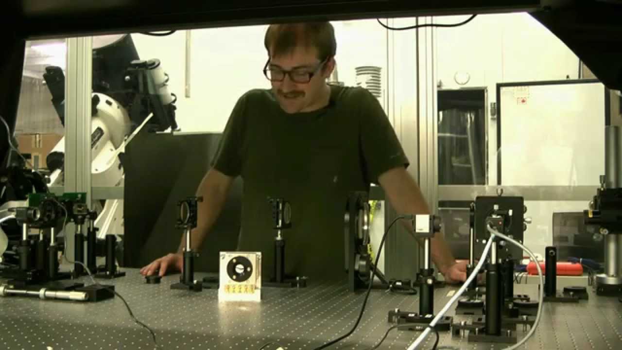
Adaptive Optics relies on wavefront sensors to measure atmospheric distortion and deformable mirrors to correct it. Wavefront sensors use grids of lenses to create reference patterns; any atmospheric aberration causes deviations from perfect alignment, revealing distortion levels. Deformable mirrors employ two main actuator technologies: piezoelectric actuators that expand/contract under voltage (creating piston-like motion) and electrostatic actuators using drum-like membranes that flex under electrostatic forces. Mirror systems typically combine a woofer (fewer actuators for coarse corrections) with a tweeter (many actuators for fine adjustments), similar to speaker systems. Small-scale prototyping is essential before building large instruments, as full-scale deformable mirrors cost millions of dollars.
Click to watch →
Peter Buschkamp: Shooting lasers into space – for science!
723
Adaptive Optics (AO) solves atmospheric distortion through three core components: a deformable mirror, a wavefront sensor, and a real-time computer operating in a feedback loop. The concept originated in 1953 at Palomar Observatory, proposing continuous measurement and correction of mirror figures to counteract atmospheric seeing. The wavefront sensor (such as the Shear-Harman type) measures how incoming light is distorted by comparing focal spot positions against a reference grid. The real-time computer processes these measurements at approximately 1 kHz to compute mirror shape corrections. This dynamic correction enables diffraction-limited imaging on the ground, matching space-based telescope quality.
Click to watch →

Adaptive Optics Human Eye
5.1K
An adaptive optics system consists of three main components working together: (1) a wavefront sensor that measures optical aberrations, (2) a deformable mirror with many independently controllable pistons that can change shape rapidly, and (3) a control system that calculates and applies corrections. The process works iteratively: light from a reference point passes through the optical system, the wavefront sensor measures distortions, the control system computes the necessary mirror shape to compensate, and the corrected wavefront produces a sharp image. This technology enables diffraction-limited imaging in both astronomical observations and retinal imaging applications.
Click to watch →

Adaptive Optics Explained: Wavefront Correction & Microscopy
4.4K
Adaptive optics is a technology that uses a deformable mirror and a Shack-Hartmann wavefront sensor to detect and correct optical aberrations in real-time; the system works by measuring wavefront distortions using a micro-lens array and camera, then calculating the mirror shape needed to restore the original wavefront, enabling applications in astronomy, microscopy, and biomedical imaging where light travels through distorting media.
Click to watch →
Deep Dive
Introductory control systems theory, particularly feedback control loops, PID controllers, and closed-loop stability.

CONTROL DE SIMULINK DESDE GUIDE de Matlab | Programación de Lazo de Control Cerrado en Simulink
3.2K
A closed-loop control system (feedback control system) consists of a reference signal (set-point), a controller that processes information, actuators that perform actions, a process or plant, and sensors that measure the output. The measured output is compared with the reference to calculate an error, which is fed back to the controller for correction. A PID controller combines three components: proportional (P) provides immediate response to current error, integral (I) eliminates steady-state error by accumulating past errors, and derivative (D) predicts future error based on rate of change to improve stability.
Click to watch →

Tutorial by Dr. Lei Zhou on feedback control loop - MIT's LabVIEW-based Dynamic signal analyzer tool
209
PID control implements three virtual elements in feedback loops: proportional gain KP creates a virtual spring between reference and measured position, derivative gain KD implements a virtual dashpot for damping oscillations, and integral gain Ki provides disturbance rejection through error accumulation. The closed-loop transfer function CL(s) = C(s)P(s)/[1+C(s)P(s)] determines system behavior, with poles at roots of 1+C(s)P(s)=0. Real poles produce converging responses, complex poles create oscillatory behavior, and right-half-plane poles cause instability. Nyquist stability requires loop gain L(s) to reach -1, with magnitude 1 and phase -180° at crossover frequency. Bode plots enable systematic design by relating crossover frequency (bandwidth) to response speed and phase margin to stability robustness.
Click to watch →
Absolute Beginners Introduction to Control Loops – Understanding Feedback, Regulation & Stability
2.5K
Control loops are essential systems that use feedback to maintain desired output parameters by continuously measuring actual values, comparing them to setpoints, and adjusting inputs accordingly; key performance metrics include load regulation (maintaining output despite load changes), line regulation (maintaining output despite input variations), and transient response (recovering quickly from disturbances without overshoot or oscillation); system stability is critical, as oscillations that persist beyond one or two cycles indicate an unstable system that cannot function reliably.
Click to watch →
MOD 20: Introduction to Control Theory
289
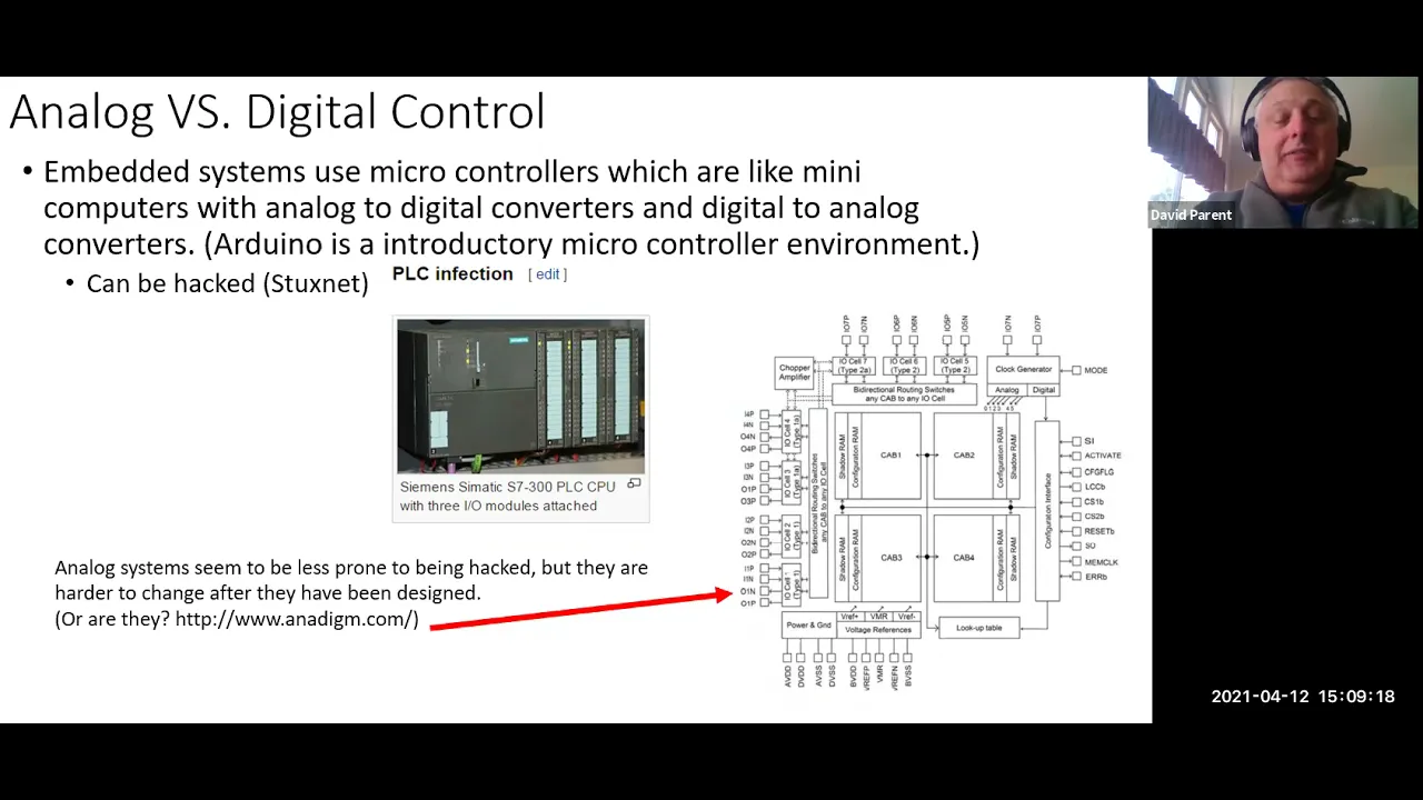
PID controllers combine three feedback mechanisms: proportional control (constant gain Kp) responds immediately to current error; integral control (K/s) eliminates steady-state error by accumulating past errors; derivative control (Ks) predicts future error based on current rate of change. The closed-loop transfer function Q(s) = H(s) / [1 + G(s)H(s)] shows how feedback modifies system dynamics, where the denominator becomes the original denominator plus the product of the original numerator and feedback network. To stabilize an unstable system, the feedback network must be chosen so all poles of the closed-loop transfer function have negative real parts. This mathematical framework enables systematic controller design, though tuning PID parameters requires careful adjustment to achieve optimal performance. The relationship between open-loop and closed-loop behavior provides the theoretical basis for understanding how feedback transforms system characteristics.
Click to watch →

PID For Robot Control Part 1
24.5K
A PID (Proportional-Integral-Derivative) feedback loop is a control system that continuously monitors a system's state through sensors, calculates the error between the current state and the desired goal, and uses a mathematical function to adjust actuators, creating an infinite loop that maintains the system at the target state despite external disturbances.
Click to watch →
Prerequisite Knowledge
- Concept 01Basic MATLAB programming proficiency, including matrix manipulation, scripting, and familiarity with toolbox environments.
- Concept 02Fundamental principles of wave optics, including wavefront aberrations, phase distortion, and optical propagation.
- Concept 03Core concepts of Adaptive Optics (AO) components, specifically the physical roles of deformable mirrors (DMs) and wavefront sensors (e.g., Shack-Hartmann).
- Concept 04Introductory control systems theory, particularly feedback control loops, PID controllers, and closed-loop stability.
Subsequent Learning
- Step 01Implementation of advanced wavefront reconstruction and control algorithms, such as Kalman filtering, modal control, or machine learning-driven correction.
- Step 02Hardware-in-the-loop (HIL) integration, interfacing the MATLAB software environment with physical optical hardware in a laboratory setting.
- Step 03Exploration of complex AO architectures, such as Multi-Conjugate Adaptive Optics (MCAO), Laser Guide Star (LGS) systems, or Extreme Adaptive Optics (ExAO).
- Step 04Application of AO control loops to specialized domains, including ground-based astronomical imaging, biomedical retinal imaging (ophthalmoscopy), or free-space laser communications.
AC Setup
Mirror Control
Closed Loop
Loop Tuning
Shutdown
AC Setup
0:00Playing Section
- 1
Initialize AC simulator and key classes.
- 2
Configure camera and wavefront sensor.
- 3
Start real-time displays for monitoring.
Limitations of MATLAB-Based Toolboxes and the Rise of Open-Source, Real-Time Alternatives
While the ACE MATLAB toolbox offers an excellent framework for simulating adaptive optics (AO), relying on MATLAB poses significant limitations for practical and real-time applications. First, MATLAB is a proprietary, costly platform, which restricts accessibility compared to open-source alternatives like Python (using libraries such as AOtools or HCIPy). Second, MATLAB's interpreted nature introduces latency, making it ill-suited for the high-frequency, hard real-time closed-loop control required in actual astronomical observation or clinical imaging; these environments demand high-performance languages like C/C++ or hardware-accelerated platforms (GPUs/FPGAs). Lastly, modern AO research is increasingly exploring machine learning-driven wavefront reconstruction and sensorless AO, which challenge the traditional linear-control and matrix-inversion models relied upon by legacy simulation toolboxes.
Deep Dive
Implementation of advanced wavefront reconstruction and control algorithms, such as Kalman filtering, modal control, or machine learning-driven correction.

Adaptive Optics in Microscopy: Practical Use of Wavefront Correctors and Control Methods
459
Adaptive Optics corrects wavefront distortions in microscopy by using deformable mirrors with electromagnetic actuators to restore flat wavefronts, improving image sharpness; two main control methods exist—image-based optimization (iterative, slower) and wavefront sensing (direct, faster)—with emerging machine learning approaches offering robust, hardware-efficient alternatives for real-time correction.
Click to watch →

OSC Colloquium: Jared Males "The Mysterious Lives of Speckles"
220
Three advanced techniques enable extreme AO performance: (1) Focal diversity phase retrieval achieves near-perfect alignment (95% Strehl) by learning system characteristics from its own measurements without pre-characterization; (2) Data-driven predictive control eliminates the need for detailed system models by learning characteristics in real-time from operational data, adapting continuously to changing atmospheric conditions; (3) Post-coronagraph wavefront sensing uses the focal plane itself as a sensor to detect and correct quasi-static instrumental aberrations, achieving 10^-8 contrast. Combined, these techniques enable detection of planets at the 10^-7 contrast level required for habitable zone terrestrial planets.
Click to watch →

Lina Streich: "High-resolution deep brain imaging using adaptive optics three-photon microscopy"
2.1K
Three main approaches exist for wavefront correction: pixelated piston-based, zonal, and modal. Pixelated approaches divide the pupil into many small subzones where phase is modulated to achieve constructive interference at the focus. Zonal approaches divide the pupil into intermediate-sized zones where tip-tilt corrections are applied before phase adjustment. Modal approaches modulate the entire pupil simultaneously using different modes with varying amplitudes. Performance depends on signal-to-noise ratio and aberration complexity: modal approaches work best for low-order aberrations while pixelated/zonal approaches handle complex aberrations with steps. Under low signal-to-noise conditions, modal approaches are more robust because modulating the entire pupil produces larger expected signal changes.
Click to watch →
Zernike Polynomial - Meeting 1 - Julia Project - CMI
706
Implementing wavefront reconstruction requires careful attention to several practical considerations. First, the Zernike polynomials must be converted from their standard polar coordinate definition to Cartesian coordinates for computational convenience. Second, the derivatives of these polynomials must be analytically computed for efficient evaluation. Third, the system matrix T must be constructed by evaluating these derivatives at all grid points. Finally, the overdetermined system is solved using least squares methods such as pseudo-inverse or singular value decomposition to obtain the best estimate of the Zernike coefficients.
Click to watch →

Claude Plymate on Adaptive Optics - Astronomical League Live - Explore Alliance
203
The Shack-Hartmann wavefront sensor uses a 2D array of tiny lenses to sample the telescope pupil and measure wavefront distortions. Each sub-aperture creates a spot image whose displacement indicates local wavefront tilt. For point sources, centroids determine offsets; for extended objects, cross-correlation techniques like Sum of Absolute Differences identify optimal alignment. Wavefront reconstruction uses Zernike polynomials—a series of mathematical modes describing physical aberrations from tip/tilt through higher-order distortions. The computer fits measurements to these modes, determining amplitude coefficients for each mode. This approach is computationally efficient because the computer learns each mode's characteristics once and then simply applies multiplicative gains during operation. The number of modes is limited by available actuators, creating a fundamental trade-off between correction quality and system complexity.
Click to watch →
Deep Dive
Hardware-in-the-loop (HIL) integration, interfacing the MATLAB software environment with physical optical hardware in a laboratory setting.
![HIL Solutions [EP.6] การประยุกต์ใช้Hardware In Loopในการทดสอบผลิตภัณฑ์โดย อ.ศุภลักษณ์ ศรีตา ม.นเรศวร](https://i.ytimg.com/vi_webp/qPLnL2q_KDw/maxresdefault.webp)
HIL Solutions [EP.6] การประยุกต์ใช้Hardware In Loopในการทดสอบผลิตภัณฑ์โดย อ.ศุภลักษณ์ ศรีตา ม.นเรศวร
297
HIL systems require separation between hardware simulation and control software. The computation block in MATLAB/Simulink contains all hardware models (power sources, filters, loads) and executes on the HIL system's FPGA. The control block contains the user interface for parameter adjustment and displays results on the Host PC. The Host PC runs MATLAB with RT-Lab software for simulation management, while the Target CPU inside the HIL system runs on Linux. The FPGA executes hardware models at approximately 200 nanoseconds per step, enabling realistic real-time simulation. Signal flow includes voltage source converter (3-phase) with LCL filter and grid connection. Signal scaling is critical: for a 5 kW system at 380V with 10.7A peak current, signals must be scaled from 3.3V DSP output to 5V HIL input, then to appropriate ranges for the DSP's ADC (16-bit, 4095 counts) to ensure maximum resolution.
Click to watch →
HIL Simulation and Testing with Simulink Real Time and Speedgoat Target Hardware
38.2K
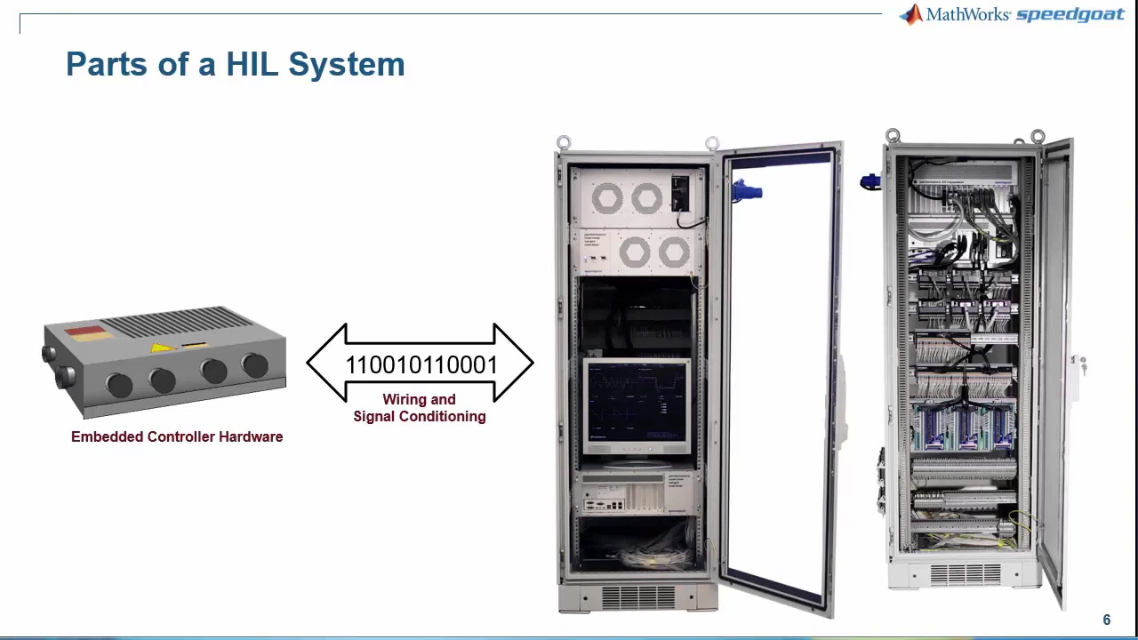
Hardware-in-the-loop (HIL) simulation integrates real-time simulation with physical hardware to verify control systems before deployment. This webinar demonstrates HIL using Simulink Real-Time and Speedgoat hardware with an oil rig draw works example where a PLC controls an induction motor and hydraulic brake. A typical HIL test bench comprises three components: the system under test (embedded hardware like PLCs), the HIL simulator hardware running Simulink Real-Time, and the test monitor. The workflow involves deploying controller models to embedded hardware, replacing them with I/O drivers for communication, and deploying the test harness. Key benefits include safe lab testing with 100% repetition accuracy, automated testing with reusable test vectors, proof of functional equivalence between simulation and deployed hardware, elimination of complex unit integration costs, ability to test dangerous scenarios without equipment damage, and easy fault injection for comprehensive system calibration.
Click to watch →
MATLAB with Physical Devices
185
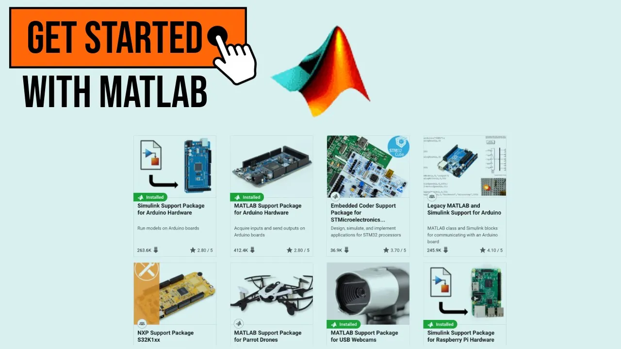
This section covers the complete setup process for connecting MATLAB with physical hardware. MATLAB offers a 30-day free trial accessible via public email, providing access to MATLAB, Simulink, and 80+ products. Two versions exist: MATLAB Online for virtual simulation and Desktop Software for local hardware connection. The RTL SDR dongle, a software-defined radio using R860 tuner and RTL 2832 chip, requires a monopole antenna for sub-GHz frequency reception. MATLAB add-ons through the Add-ons tab provide hardware support packages. After connecting hardware via USB with PoE power, proper drivers must be installed using tools like Zadig for RTL SDR devices. This setup enables communication between MATLAB and physical devices for real-time signal processing and analysis.
Click to watch →

Capstone Final Year Project 3: MATLAB Simulink Hardware in Loop (HIL) Setup using FPGA
221
Hardware-in-the-Loop (HIL) testing enables rapid prototyping of controllers and converters by deploying Simulink models onto FPGA hardware, allowing real-time testing of complex control algorithms like PID controllers without building expensive physical hardware; the setup requires compatible MATLAB and Vivado versions, proper installation of HDL Coder support packages, data type conversion for 32-bit JTAG communication, and verification that FPGA deployment produces results matching pure simulation.
Click to watch →

MIL SIL Tutorial: Part 5
6.2K
Hardware-in-the-Loop (HIL) simulation involves building a real-time model using Real Time Workshop, configuring input control through constant blocks and from workspace signals, unchecking block reduction for HIL compatibility, selecting the appropriate target file for the hardware platform, and generating HIL files for hardware testing with subsequent result analysis in MATLAB.
Click to watch →
Deep Dive
Exploration of complex AO architectures, such as Multi-Conjugate Adaptive Optics (MCAO), Laser Guide Star (LGS) systems, or Extreme Adaptive Optics (ExAO).

PSW 2447 Twelve Times Hubble and Halfway to Space | Fengchuan Liu
971
Adaptive optics corrects atmospheric distortion by measuring wavefront aberrations in real-time and commanding deformable mirrors to compensate. The system uses wavefront sensors and controllers operating at ~600 Hz. Since natural guide stars aren't always available, laser guide stars excite sodium atoms at 90km altitude to create artificial reference points. Multi-conjugate AO uses two deformable mirrors conjugated to different altitudes (ground layer and 11km) for volumetric correction. Canada provides the multi-conjugate AO instrument with deformable mirrors having 3,100+ and 4,500+ actuators respectively. The system accepts AO-corrected light through beam transfer optics from below the primary mirror to the top end. This technology enables diffraction-limited imaging, transforming ground-based telescopes into competitive instruments for high-resolution astronomy.
Click to watch →

Lorenzo Busoni - Multi Conjugate Adaptive Optics for Extremely Large Telescopes
419
Multi-Conjugate Adaptive Optics (MCAO) is an advanced technique that uses multiple deformable mirrors, multiple wavefront sensors, and multiple reference sources (both natural guide stars and laser guide stars) to provide three-dimensional correction of atmospheric turbulence across a wide field of view, enabling Extremely Large Telescopes (ELTs) with 25-40m diameters to achieve diffraction-limited imaging performance; this approach addresses the fundamental challenge that single-conjugate AO systems can only correct atmospheric turbulence effectively near the ground layer, while MCAO extends correction to higher altitude layers through tomographic reconstruction of the atmospheric phase perturbation.
Click to watch →

The ITSO/AAO OTW2016: Adaptive Optics by M. Goodwin
102
A complete AO system consists of wavefront sensors, deformable mirrors, high-speed control systems, and science cameras. The Shack-Hartmann sensor uses lens arrays to sample wavefronts, creating spot patterns indicating local slopes. Deformable mirrors with piezoelectric actuators correct distortions by moving a few microns at high frequencies. Multi-object AO (MOAO) extends this to observe multiple targets simultaneously using multiple wavefront sensors and deformable mirrors. Laser tomography uses multiple guide stars to sample atmospheric turbulence at different altitudes, enabling multi-conjugate AO (MCAO) that corrects different atmospheric layers. Single-mode waveguides and polymer bundles enable efficient multi-object observations by guiding light from multiple targets to single detectors.
Click to watch →
4. Atmospheric Turbulence and Solar Adaptive Optics - Jose Marino
468
Multi-conjugate adaptive optics extends correction to wider fields by using multiple deformable mirrors conjugated to different atmospheric heights where distortions originate, requiring tomographic reconstruction of the 3D atmospheric structure using multiple wavefront sensors. This achieves ~60 arcsecond field correction compared to classical AO's narrower region. Modern implementations use parallel computing with multi-core CPUs rather than dedicated hardware, enabling real-time processing of thousands of cross-correlation calculations per frame. Despite complexity, complete correction remains challenging due to the 3D nature of atmospheric turbulence, with residual distortions affecting data analysis for applications requiring multiple exposures or time-series measurements.
Click to watch →
Chapter 8.4 Adaptive optics and large telescopes - II
127
Adaptive optics (AO) systems compensate for atmospheric distortion to achieve diffraction-limited imaging. Key components include wavefront sensors measuring instantaneous distortions, computers calculating phase errors, and deformable mirrors correcting shapes. The process involves measuring spot locations, calculating slopes between adjacent spots, and solving linear equations to reconstruct wavefronts. Atmospheric turbulence changes rapidly at millisecond timescales, requiring AO loop closure rates of 1 kHz or higher. Finding sufficiently bright natural guide stars within small angular separations from arbitrary targets is statistically unlikely. Solutions include laser guide stars tuned to sodium transitions at 90 km altitude, creating artificial stars. However, laser guide stars cannot measure overall tip-tilt motion due to atmospheric refraction. The cone effect further limits single-laser systems, requiring multi-conjugate AO with multiple lasers and wavefront sensors for large telescopes. AO performance is measured using full width at half maximum (FWHM) comparing image angular size to the diffraction limit (λ/D), and the Strehl ratio measuring peak intensity relative to theoretical maximum. Telescope sensitivity scales approximately with D^4, meaning a 2-meter telescope with AO is 16 times more sensitive than a 1-meter telescope. Extreme adaptive optics combines coronagraphs blocking starlight with powerful AO systems suppressing scattered light, enabling direct imaging of exoplanets.
Click to watch →
Deep Dive
Application of AO control loops to specialized domains, including ground-based astronomical imaging, biomedical retinal imaging (ophthalmoscopy), or free-space laser communications.
ALPAO Webinar Adaptive Optics for Free Space Optics Communication
2K
Free space optics (FSO) transmits light through unguided media like air or space without fiber optics. The satcom market, a major FSO segment, grew to $23B in 2018 with 7% annual growth projected to $41B. Atmospheric turbulence degrades FSO links by distorting wavefronts, causing signal fading. Adaptive optics (AO) corrects this by using a deformable mirror controlled in closed-loop with a wavefront sensor. The system flattens distorted wavefronts, concentrating energy into smaller spots for improved communication quality. This same principle applies to both astronomical imaging and FSO applications.
Click to watch →

Intro2Astro 2024: Adaptive Optics
105
Guide stars provide reference points for measuring atmospheric distortions in AO systems. Natural guide stars are bright stars near the target, while artificial guide stars are created using laser beacons that illuminate sodium atoms in the upper atmosphere, causing fluorescence. These guide stars experience the same atmospheric turbulence as the astronomical target, enabling accurate measurements. AO has expanded beyond astronomy into multiple applications: ophthalmology uses it for retinal imaging without aberration, microscopy employs it for deeper focus and aberration correction, free-space optical communications use it to correct turbulence-induced distortions in data transmission, and lasers with AO enable precise beam shaping for atomic trapping, laser cutting, quantum computing, and precision manufacturing. In astronomy, AO enables high-contrast imaging for directly detecting exoplanets and circumstellar disks, combining AO with coronagraphy and post-processing techniques to distinguish faint planets from stellar speckles.
Click to watch →
Intro2Astro: Adaptive Optics
144
Adaptive Optics (AO) revolutionizes imaging by correcting atmospheric distortions that blur ground-based observations. Stars twinkle due to atmospheric turbulence causing refraction and wavefront distortion. AO systems use deformable mirrors (segmented, piezoelectric, continuous, or MEMS types) to counteract these distortions in real-time. Key components include wavefront sensors (Shack-Hartmann and pyramid types) that measure aberrations and guide stars (natural or laser-created) as reference points. AO enables high contrast imaging for exoplanet detection and extends to applications in vision science, microscopy, free space optical communications, and laser technology for precision manufacturing and quantum computing.
Click to watch →
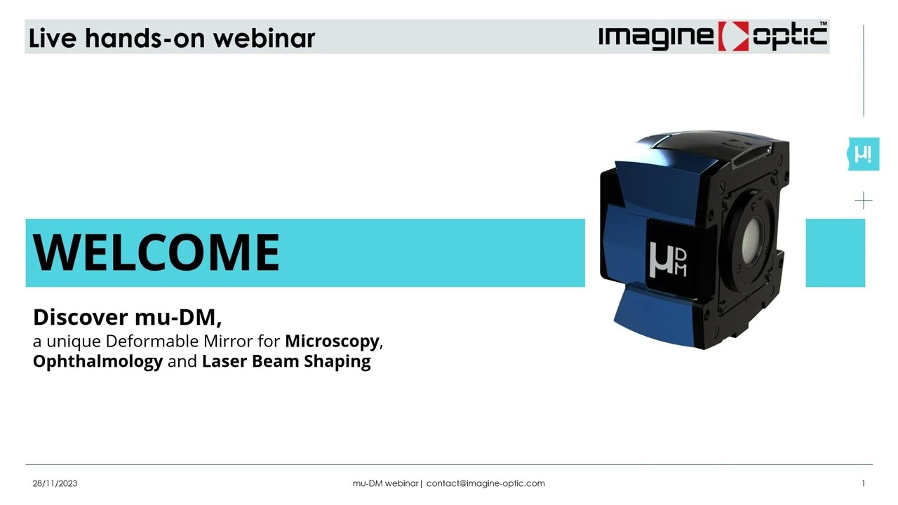
WEBINAR - Adaptive Optics - LIVE DEMO - New Deformable Mirror 'mu DM'
628
Adaptive Optics corrects wavefront aberrations degrading biological imaging. In fluorescence microscopy, scattering, absorption, and aberrations distort images, with aberrations causing signal loss and resolution degradation with depth. In ophthalmology, the cornea and crystalline lens introduce aberrations limiting retinal imaging. Two correction approaches exist: direct wavefront sensing (Shack-Hartmann sensor + deformable mirror in closed-loop) offers high accuracy (λ/100) but requires dedicated light and complex setup; sensorless AO uses only a deformable mirror with iterative image-based optimization, simpler but slower. Closed-loop suits dynamic samples and high accuracy; sensorless suits static samples. Four phase modulation technologies serve these needs: liquid crystal spatial light modulators, deformable mirrors, transmissive adaptive lenses, and electromagnetic deformable mirrors. For life sciences, key requirements include sufficient actuators for high-order aberration correction, adequate stroke amplitude (tens of microns for ophthalmology), high linearity for rapid convergence, temporal stability over hours, compact integration, and improved price-performance.
Click to watch →

Chapter 8.4: Adaptive optics and large telescopes – II | A N Ramaprakash
205
Adaptive optics (AO) systems compensate for atmospheric turbulence that degrades astronomical images. The system uses a wavefront sensor to measure instantaneous wavefront distortions, calculates slopes at each aperture, determines phase errors, and generates signals to deform a mirror in real-time. Without AO, starlight appears as scattered blobs; with AO activated, light concentrates into a sharp Airy disk matching the telescope's diffraction limit. Atmospheric changes occur on millisecond timescales, requiring AO loops operating at kilohertz frequencies or faster for large telescopes.
Click to watch →
AC Setup
Mirror Control
Closed Loop
Loop Tuning
Shutdown
AC Setup
0:00- 1
Initialize AC simulator and key classes.
- 2
Configure camera and wavefront sensor.
- 3
Start real-time displays for monitoring.
Limitations of MATLAB-Based Toolboxes and the Rise of Open-Source, Real-Time Alternatives
While the ACE MATLAB toolbox offers an excellent framework for simulating adaptive optics (AO), relying on MATLAB poses significant limitations for practical and real-time applications. First, MATLAB is a proprietary, costly platform, which restricts accessibility compared to open-source alternatives like Python (using libraries such as AOtools or HCIPy). Second, MATLAB's interpreted nature introduces latency, making it ill-suited for the high-frequency, hard real-time closed-loop control required in actual astronomical observation or clinical imaging; these environments demand high-performance languages like C/C++ or hardware-accelerated platforms (GPUs/FPGAs). Lastly, modern AO research is increasingly exploring machine learning-driven wavefront reconstruction and sensorless AO, which challenge the traditional linear-control and matrix-inversion models relied upon by legacy simulation toolboxes.
Basic MATLAB programming proficiency, including matrix manipulation, scripting, and familiarity with toolbox environments.
Fundamental principles of wave optics, including wavefront aberrations, phase distortion, and optical propagation.
Core concepts of Adaptive Optics (AO) components, specifically the physical roles of deformable mirrors (DMs) and wavefront sensors (e.g., Shack-Hartmann).
Introductory control systems theory, particularly feedback control loops, PID controllers, and closed-loop stability.
Implementation of advanced wavefront reconstruction and control algorithms, such as Kalman filtering, modal control, or machine learning-driven correction.
Hardware-in-the-loop (HIL) integration, interfacing the MATLAB software environment with physical optical hardware in a laboratory setting.
Exploration of complex AO architectures, such as Multi-Conjugate Adaptive Optics (MCAO), Laser Guide Star (LGS) systems, or Extreme Adaptive Optics (ExAO).
Application of AO control loops to specialized domains, including ground-based astronomical imaging, biomedical retinal imaging (ophthalmoscopy), or free-space laser communications.
1.3K views6likes9:00@adaptiveopticsOriginal Release: 2015-03-27
welcome to the AC tutorial here we will present the Matlab AC toolbox firstly we initialize the AC simulator in Matlab AC is based on an object orientated environment DM represents the de the deformable mirror class and here we can see all its Associated functions the function online switches on the deformable mirror Loop is also an object here we can see its Associated functions next we will introduce the camera control the camera is initialized by using Cam and and the function online next we set the integration time and the gain for the camera we can monitor the camera by starting the real-time display next we will look at the wfront sensor we turn on the wfront sensor by typing wfs online we can get the center of gravity for each micr lens and then plot it the phase can also be extracted and then can be plotted to an image we can also extract the xeri vectors which the wavefront is composed of we can also monitor the slopes of the wavefront sensor by starting the slope realtime display the measured wavefront can also be monitored to initialize the system we get the measured slopes from the wfront sensor and we set these slopes as a reference measurement next we will look at the control of the deformable mirror first we turn on the deformable mirror and we start the monitoring of the mirror like so before anything else we reset the mirror here we extract the number of actuators of the deformable mirror in order to actuate them one by one in order to verify that all the actuators are functioning correctly we actuate each one in turn instead of actuating each actuator in turn we can also send a vector of commands to the deformable Mirror in this manner we can send whichever shape we choose the mirror can also be controlled using the xeri mode basis here we introduce some defocus in the mirror and we can verify our modes by getting the phase from the wfront sensor as well as the xeri modes we finish once again by resetting the different mirror next we will look at combining all three elements in the Clos Loop we turn on the loop like so here we Define the parameters which are used to measure the influence Matrix the influence functions of the formable mirror are measured by pushing and pulling each actuator in turn and measuring their influence on the wfront sensor then the command Matrix is calculated for the desired number of of modes and the xeri 2 command Matrix is also extracted from this now we can start the monitoring of the loop first we set the reference slopes next we Define a perturbation which is in this case a defocus and we apply this to the incident beam after defining the gain we close the loop to compensate for the perturbation as we can see on the display the wfront is flattened and the resolution is is improved as the mirror shape compensates for the perturbation the loop can also compensate for any random perturbation as we show here to change the properties of the loop we first open the loop and reset the mirror now we can increase the gain of the loop in order to increase the correction speed once again we close the loop and as we see on the real time display the correction is much faster finally we switch off all the elements of the loop thank you for watching
Up Next

13:54
AMD CEO Lisa Su on High Performance Computing Vision
@SixFiveMedia
93.6K views•2021-06-17

12:54
Triumph of Orthodoxy Icon: Byzantine Art & History Explained
@BenCallan
2.1K views•2024-08-06

9:49
FastAPI vs Flask vs Django: Choosing the Right Python Web Framework
@TechWithTim
302.5K views•2024-05-26

1:42
Game of Thrones Opening Credits: A Cinematic Analysis
@gameofthrones
46.3M views•2011-04-18
Related Study Plans & Knowledge Roadmaps
Structured learning paths in General & Interdisciplinary Studies
general-studies
Elevator Engineering: History, Physics & Cities
01From Hoists to Safety Brakes: The Dawn of Vertical Lift
02Hydraulic vs. Traction: The Engineering Physics of Elevators
03Modern Speed, Safety, and Algorithms
+ 2 more learning modules
12h5 modules
Explore Roadmap
general-studies
Rubber: Material Science, History & Geopolitics
01Origins of Natural Rubber & Mesoamerican History
02The Chemistry of Natural Rubber & Vulcanization
03The Geopolitics of the Rubber Boom & Colonization
+ 2 more learning modules
12h5 modules
Explore Roadmap
general-studies
Containerization: Evolution, Logistics & Trade
01Ancient Trade & Bulk Cargo: Amphorae to Barrels
02The Industrial Revolution & Cardboard Packaging
03The Containerization Revolution: Malcom McLean
+ 2 more learning modules
12h5 modules
Explore Roadmap
general-studies
Textile Tech: Evolution, Labor & Global Impact
01Pre-Industrial Textiles: Handloom & Cottage Industry
02Mechanization: The Spinning Jenny to the Power Loom
03The Factory System & Global Labor Transformation
+ 2 more learning modules
10h5 modules
Explore Roadmap