



















This tutorial demonstrates how to use two Active Optical Systems tools—the Beam Control Scaling Law tool and the Control Simulator—to estimate atmospheric propagation characteristics (including Fried's coherence length r₀, Greenwood Frequency fG, Isoplanatic Angle, and Rytov Number) and determine the compensation capability of tilt and adaptive optics systems. The Beam Control Scaling Law tool calculates required system parameters such as actuator count, bandwidth requirements (e.g., 45 Hz tilt bandwidth and 300 Hz AO bandwidth for a 20 cm aperture at 1 km range), and laser power requirements based on input parameters like platform altitude, aperture diameter, wavelength, wind velocities, and target location. The Control Simulator tool then estimates control bandwidths (-3dB error rejection transfer function, unity gain ERTF, and -3dB closed-loop transfer function) using engineering parameters including sample rate, latency, and gain, enabling designers to evaluate system performance before implementation.
Beam Control Scaling Law & Control Simulator Tutorial
Added:Hi, I'm Justin Manel from Active Optical Systems and this is a tutorial on how to use the AOS beam control stealing law code and the control simulator tool.
So, you can get these tools by going to the AOS website and going to the bottom here and clicking on the link to the SharePoint site. The AOS website is www.aoslc.com.
You click on that, it will then take you to the AOS SharePoint. I've already logged in today, so it was a very quick load. If you haven't logged in, it's a much slower load usually. Then you can click on downloads, export controlled software, utilities, and the two tools I'm talking about today are the beam control scaling law tool and the control simulation tool. Okay? Okay. So once those are downloaded and installed and that may require you to uninstall the old versions if you have them on your computer now you can move on to actually running them. So once I've done that um I can go into let's start with this one. This is the generic how do you simulate a beam control system tool.
So what you can do with this is specify a platform altitude. So basically height above the ground target altitude range and aperture diameter let's say it's 20 cm and wavelength in nanometers I'll leave it at one micron um actually a lot of the lasers that that literature there and once you have that it will then calculate parameters about the engagement so these are things like r d by rum the defraction limited spot diame diameter on target and these kinds of things. And so you can take a look at all of these, but what you can do is use this then to assess how much of an AO system and tilt system you need for this uh to compensate the aberrations. So you also can specify wind velocities. By the way, I forgot to mention that. And specify the wind uh the platform velocity and the target velocity. Um those are used to derive greenwood frequencies and tilt greenwood frequencies for your system. Okay. So then you can use the simulator tool to take a look at how much of a tilt system you need. So this is a 10 herz tilt system. Um again this is a 1x HP57. Um and so with a a 10 herz system we're not going to get perfect compensation. We're only going to get about 65 let's see 66% compensation there. Let's see if we can speed that system up um to 30 Hz. Good.
So this is a 30 Hz system and now we're getting um you know 80% tilt uh compensation. So this is a pretty good system. Um one of the things I'm not addressing in any of this is what happens when uh how do you get this 3dB bandwidth and what does that really mean? It's the 3dB error rejection transfer function. The next tool I'll discuss how you can calculate what that is using basic parameters in your system.
On the AO side um take a look here. We were looking at d by r of three for this. Um kind of boring, not quite enough there. So let's bring up the 57 multiplier to 4x. There we go. Now we're at d by r about seven. Um which also uh affected our requirements for tilt, but let's just leave that one there. Um, and this is estimating with a 5cm R not in big beam space that I'm going to have about 13 actuators um over the full aperture. Not quite enough. I think I'm going to want something more like in the 30s. Let's make this about 2.5 cmters.
Uh, okay, that's good enough. We're in the 50s now. That's that's okay. Um and with a 300 htz um bandwidth uh we're seeing pretty good compensation here. So this is the this line indicates where you are. Um and this is the spatial term and then this is a temporal term. So temporal is a little better than spatial. Um let's see if we can actually add some more actuators. Then just make it 2 cm. There we go. Now they're both crossing over in the 80 83ish% for each of them for that one. And when you combine those, you're going to get 70%. So this system with 79 actuators and a 300 Hz 3D bandwidth looks like it's going to work well here. Um I'm going to bring this bandwidth up a little bit here.
Somewhere into the 70s I think would be good. There we go. So 45 hertz there.
So this you know in order to compensate um light propagating from a 20 cm aperture 1 kilometer 3 meters off the ground um with a 4xh 57 atmosphere and a 4% wind velocity one micron light would need uh to get decent compensation 45 hertz tilt bandwidth 300 htz AO bandwidth um and that's the 3dB bandwidth for both of those and I'll like I said I'll discuss what how you get the 3D with the other simulator and um a roughly 2 cm or 79 actuator DM 2 space.
Okay. Um there's another tool built into here that's in its early early draft phase. Um and you can go through and calculate how much of a laser you're going to need for this. This is predicting a 35 watt laser requirement.
And there's a lot of parameters to this including you know loss per path losses is percent loss per kilometer target reflectivities system loss factors quantum efficiencies um noise electrons read noise electrons pixels per spot whether we doing shackartman or whether we're doing tracking kind of things um pulse periods uh goal signal to noise ratio and target sizes. So uh once those are all specified um you can calculate what you expect for requirements for an illuminator. So now uh we can take a look at the wind velocity. This one happens to be very boring because I said that the platform target moving m crosswind. Um this is a summary of all the results about the engagement.
Um this is a graphical summary of that summary of all the key parameters like d by r not which is on the order of seven.
Um this is the rit number about 0 2.
This is the fraction limited spot uh angle versus the isopatic angle. Um and that's close to one. Um so that's getting pretty bad there. Um the tilt Greenwood frequency. So this is about how fast a tilt system uh we would need.
And uh this is the in order to get start to get good compensation. Um and then this is the uh Greenwood frequency. It's about 100 hertz. Um, and you can see we need to be a little bit above those to get significantly improved compensation system. Okay, there's another piece of this. There's there's a whole tab on here on conversions. Often times we get, you know, units that are funny and people say, "Oh, I I want to be moving at 23 knots." Well, if you type in 23 knots, it'll say that's really 12 meters a second or 26 miles an hour. That kind of thing. So, there's a bunch of conversion things that are in here.
um you can actually go through and get altitude locations out of the database.
Uh but let me go through that and explain how that works. So um with this you can go into Google Maps and start specifying locations. And so I'm going to zoom out. I'm in Albuquerque, New Mexico here. I'm going to say let's pretend like we were testing out here in the mountains. Um you can see that if you zoom out a little bit, you can start to see the contours as I zoom in a little lose them. So, I'm going to just go to satellite mode here. And what you want to do is find a a spot. We'll just say this little here. Center it up in the screen. Zoom in on it and say, "Okay, this is my platform location." And say, "Map, copy." It will copy the longitude and latitude for that location. Now, I can zoom back out and say I wanted to shoot down here um to the front of this hill. Let's say I was shot here.
uh to the front of this hill.
I've copied that as well. Then you click use location. And what it's doing now, as you can see in this progress bar, is it's going off and pulling uh one of the US government databases for altitude along there to try to figure out what the real altitude is for this engagement. This takes a few minutes and it does require that you have uh internet access for it. Um the buttons here allow you to fix some of the common errors that occur when you are using um a computer that without the the necessary explorer details on it. But you can see it came back here and it's giving me a little snapshot of my platform and my target location and it's showing me the altitude, the actual altitude and the relative altitude along there. Um, and so you can see it's rapid drop off. Got a little bump here. Um, and probably this hill here maybe. Um, and then um, it get closer and closer to the ground as we approach the target.
Okay. So with this I can go and take a look at what an engagement in real kind of environment might be. You can see here that now the CN squared plot is mimicking that altitude behavior. That makes sense. But you can see what happened here. The R not value dropped.
Uh let's see the AR not value uh increased a little bit. Now by R is more like 6.1 back summary 6.2. Okay. So now uh because I'm using real locations it's not as bad. It also filled in for me the ground range. Now the the ground range got significantly longer. I was at 1 kilometer before. Um and when I picked this range now we're at 1.6 km. But even getting with this increase in length, I had a decrease in R not. And this had to do with the fact that I'm shooting much higher off of the earth floor than I was in the previous one. Now, um that this does take into account the curvature of the Earth and in fact uh it'll plot up for you the curvature of the earth below here.
but uh it it uh does not um necessarily limit your ability to uh shoot um uh if you're not using a real engagement.
Okay, so here we go. Uh I've got the map coordinates. I've got a plot of the altitude. Um and with that, I can actually start predicting what kind of an AO system might be in a real engagement. Um I think that's basically it for this tool.
This tool allows you to do some real quick calculations as to how much of an AO system you would need in order to do a certain job.
And the only thing I didn't cover was how I got to these 3dB bandwidths for adaptive optics and for tilt. So, there's another tool we have that can help cover this. Um, actually, there's one more thing I should say here, and that is that there's a save results button. Uh, and a save button. Save here allows you to save out to your desktop or wherever actually. Uh an XML file that you can load back up. Um save results allows you to take save all of the results files out. So let me do that real quick. Hold on. Okay, so I've saved a results file out to my desktop. Let's take a look. So um it not just saves out the results file, but it also saves out a whole bunch of images and things like this. Um it basically goes through the program and saves out all the images that are available and and that kind of thing. Um this is a plot of the AO results. Um this is a plot of that wind velocity. Um this is the summary that we're showing you that shows you summary of the engagement parameters.
Um let's see. And it saves out a bunch of these AOS picture boxes as well. Um, but a lot of these are very good plots for putting into presentations. So, you save that as all those out. And I can open this up. Um, and you can see here, this is just a big XML file of all of the the various parameters of the system that could be loaded back into the system with a load operation in order to get back to the same settings you had before. Okay, so that's how the beam control scaling law system works. Now, we can talk a little bit about another piece of this.
delete all these old files that good. Now we can talk about this control simulation software. So once that's installed, you can open it up and what it's doing is trying to take some engineering parameters and determine what bandwidth for the system might be.
So it's a real simple tool, excuse me, a little simple tool. uh you can specify a sample rate, the latency and the gain and quickly calculate um what the error rejection transfer function and closed loop transfer function would look like.
Uh it's important for this tool to be running it as an administrator. If not, you're going to get a couple of bugs saying, "Hey, I can't save out the the data for this." So, let me take a second fix that.
Okay, so I ran this as administrator.
Now, I can save this out. Um, you can see that with these specifications, um, I've got a very small overshoot, meaning that I'm probably nowhere near the optimal gain on this. So, I can go in here. Let's just, because it's a nice round number, work with a 1 kilohertz rate here. Um, let's bring this latency down to say 1,000 microsconds or one millisecond. Let's bring this guy back up say.
All right. So, I'm leaving auto range on this. Uh, but you can turn that off and specify the frequency range you want to scan over. Um, you can see here that I've got a 3dB. In fact, I'm going to do a high resolution version.
And let's change this to let's do 300 points.
All right. What it's doing actually is a uh temporal simulation and reporting the results from the temporal simulation in the background. It does take a little it's more computationally intensive than a frequency approach but it can be a little more accurate. Um so let's take a look at what's coming out of this. The red curve here is the error rejection transfer function and the key parameters for that are usually when it crosses over the minus 3dB point which according to this is about 57 hertz that makes sense I expect a factor of 20 between the sample rate in a well tuned system between the sample rate and projection saying 57 that's pretty close and another commonly quoted parameter for control system like this is the crossover at zero dB which for us is about 89 hertz and then the final one that's commonly quoted is 3dB full which is 156 hertz okay so uh that's the 3dB there and it's much further out so you can see that there are three effective bandwidths that are specified or or resulting from this simulation and when you're designing your system uh used with the scaling law. This one, this 3db error rejection is what we use there. So you can go through here and specify the sample rate of your camera or or sensor.
Specify the latency. This is usually how much time it takes to not only integrate uh it's usually half the integration time, but also um how long it takes to calculate a new command. And you can specify a gain here. Um you don't want to get too high with the gain. it'll go unstable. U but 7 is a reasonable number there as well.
So I'll do another high resolution calculation. There we go. So now we're getting 60ish hertz. You can see I up the gain. Now the the bandwidth went up and the overshoot went up as well. Um okay. So this tool is very nice for determining um what these bandwidths these 3dB bandwidths are of the error rejection transfer function from engineering parameters. So those are two tools that we use to calculate requirements for adaptive optics and tilt control systems to compensate aberrations in the atmosphere. If you have any comments or questions, don't hesitate to contact us.
Thank you very much for listening.
Up Next

The Jasons: Secret History of Science's Postwar Elite
@MicrosoftResearch
41.2K views•2016-09-07

Triumph of Orthodoxy Icon: Byzantine Art & History Explained
@BenCallan
2.1K views•2024-08-06
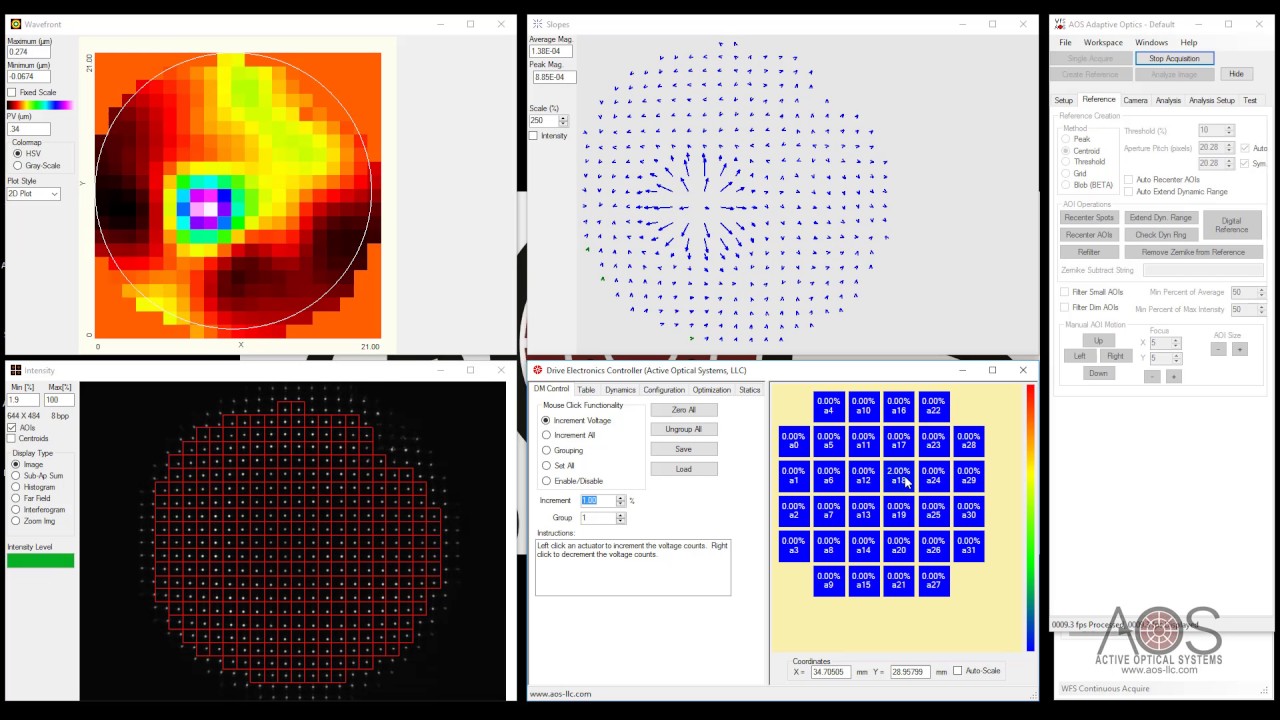
AOS Adaptive Optics System and Software Setup Tutorial
@activeopticalsystemsllc359
674 views•2017-01-02

Game of Thrones Opening Credits: A Cinematic Analysis
@gameofthrones
46.3M views•2011-04-18
Related Study Plans & Knowledge Roadmaps
Structured learning paths in General & Interdisciplinary Studies