





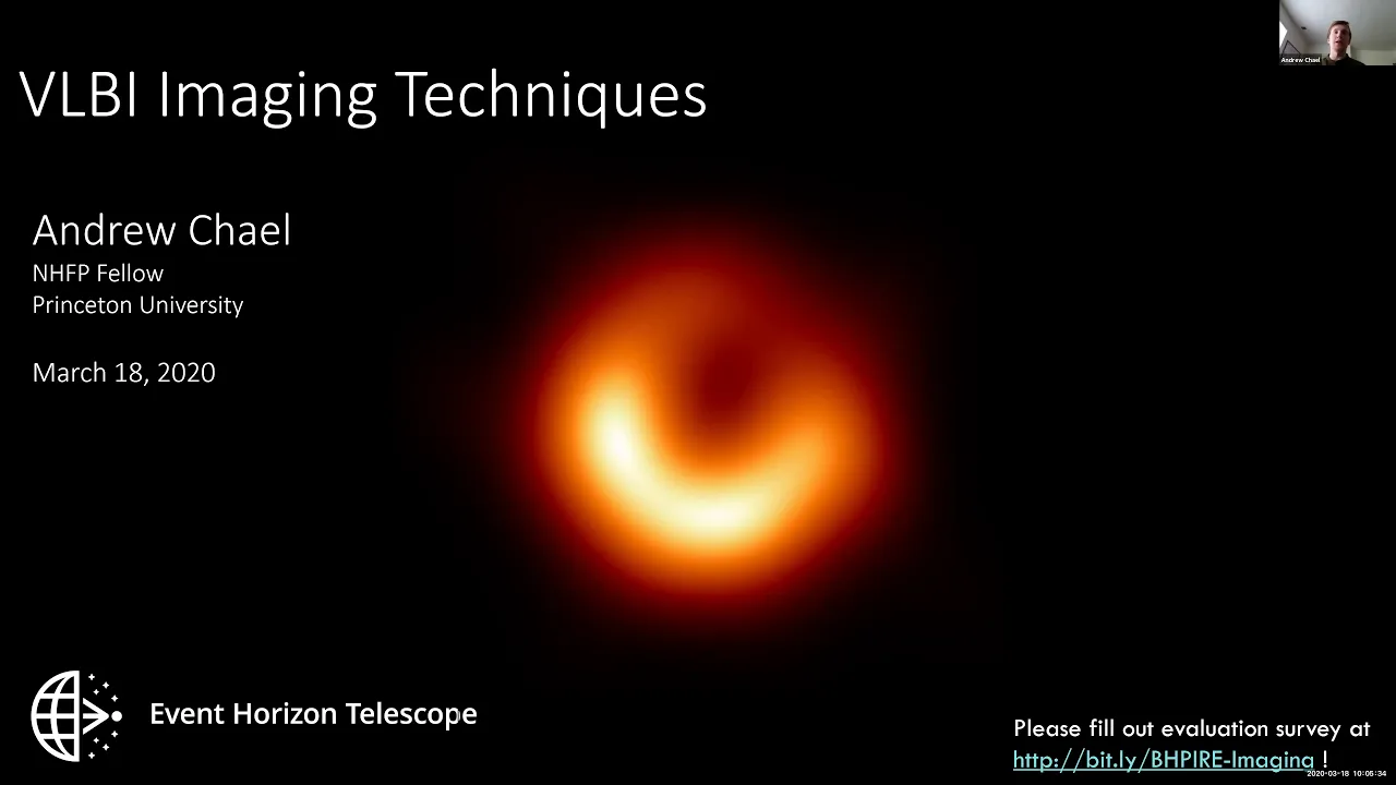






The CLEAN algorithm, developed by Ronald Hogg in 1974, is the standard method for reconstructing astronomical images from radio interferometry data by iteratively deconvolving the dirty beam from dirty images; the algorithm works through nested major and minor cycles where minor cycles perform image-plane deconvolution to add clean components to the model, while major cycles transform back to the uv plane for accurate subtraction, balancing computational efficiency with image accuracy.
ALMA Primer: How the CLEAN Algorithm Deconvolves Interferometric Images
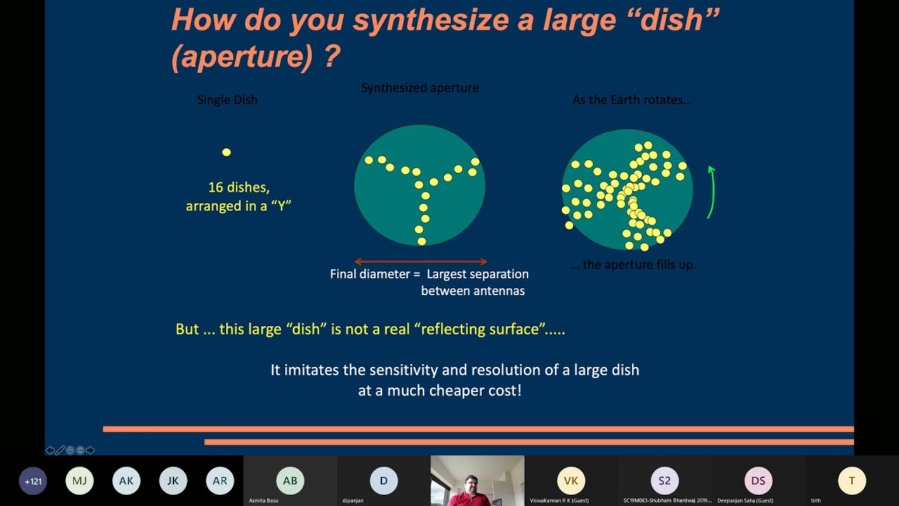
Added:Fundamentals of radio interferometry, including baseline configurations and the concept of the uv-plane.
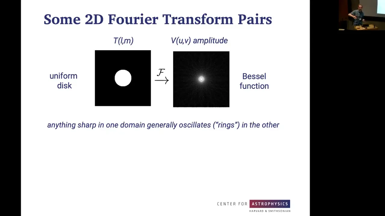
The relationship between visibility data and sky brightness via the 2D Fourier Transform.
The concept of 'dirty images' and the Point Spread Function (PSF) or 'dirty beam' resulting from incomplete uv-coverage.
Basic mathematical concepts of convolution and deconvolution in image processing.
Advanced variants of the CLEAN algorithm, such as Multi-Scale CLEAN and Multi-Frequency Synthesis (MS-MFS) CLEAN.
The process of Self-Calibration, using CLEAN-generated sky models to correct systematic phase and amplitude errors.
The impact of visibility weighting schemes (Natural, Uniform, and Briggs/Robust weighting) on the PSF and resulting CLEAN images.
Alternative and modern reconstruction techniques, such as regularized maximum likelihood (RML) imaging and compressive sensing.
2.3K views83likes8:14Original Release: 2022-08-02
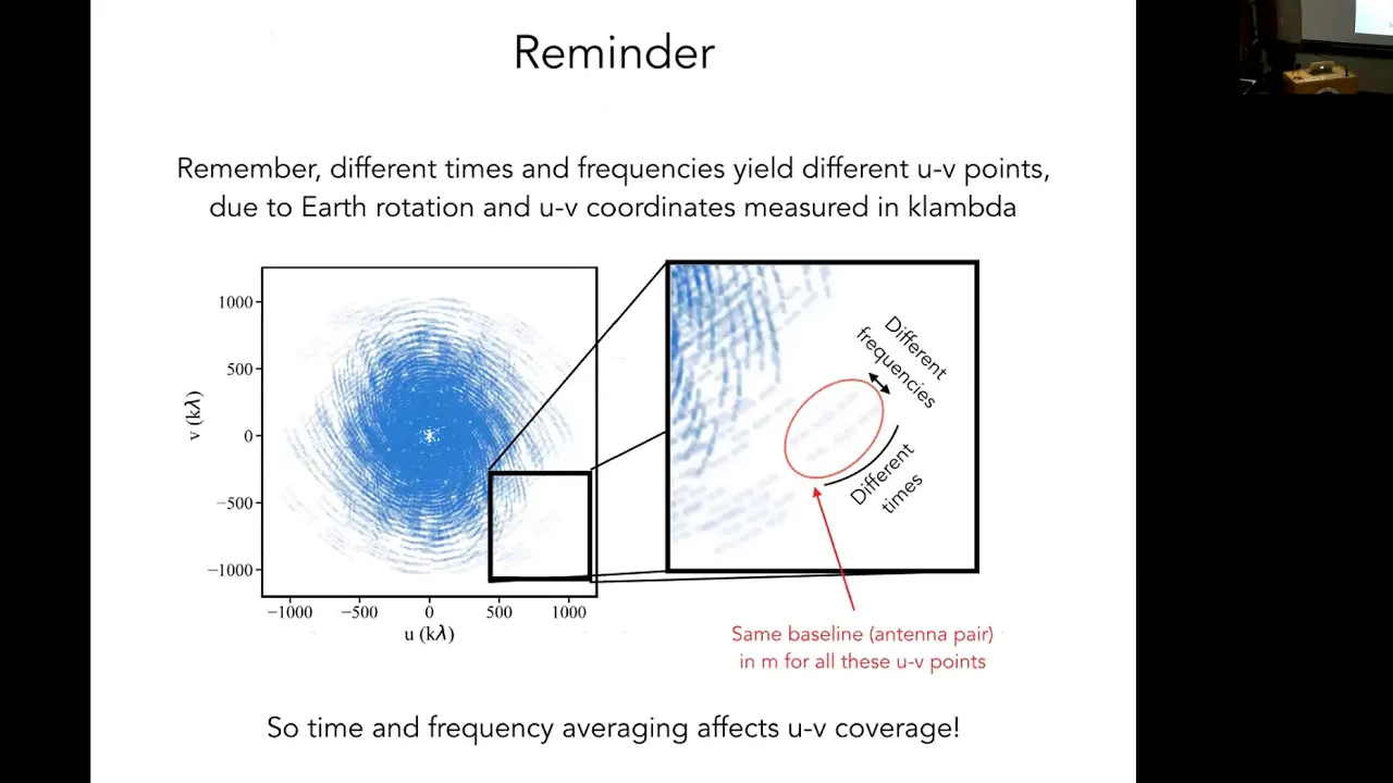
in this video we'll discuss clean a commonly used approach for reconstructing images from radio interferometry data like from alma as we've discussed in other videos the data collected by an interferometer are called visibilities which are the fourier transform of the sky brightness distribution measured for each pair of antennas while you can analyze the visibilities directly to do your science typically you want to convert the visibilities into an image you might think we could simply inverse fourier transform the visibility data to produce an image but because the measured visibilities only sample a discrete portion of the uv plane transforming into the image plane introduces ringing side lobes and general messiness into the image mathematically we can represent this by multiplying the fourier transform of the true brightness distribution by a sampling function which is only non-zero where we measure the power spectrum when we transform our incompletely sampled data back into the image plane the convolution theorem tells us that the result will be the brightness distribution convolved with the fourier transform of the sampling pattern this fourier transform of the sampling pattern is called the point spread function or psf of our image and in radio astronomy we call it the dirty beam the images we produce by directly transforming visibility data are called dirty images here are a few examples of dirty images and their corresponding dirty beams to recover the true sky brightness distribution we want to deconvolve the dirty beam from the dirty image in order to produce a model which best approximates the true sky brightness there are different ways to approach deconvolution in order to compensate for the incomplete uv sampling but one of the most robust is the clean algorithm which was first published by yong hogbam in 1974.
clean uses an iterative approach to derive a model of the true sky brightness after a dirty image is made the clean algorithm identifies the brightest position in the map and adds a single point source to the model at that location we refer to this point source as a clean component the amplitude of this component is equal to the brightness at that location in the map multiplied by a gain factor of less than one to account for the fact that in the real map the brightness at that location is most likely the contribution of multiple sources plus noise the next step is to convolve this component with our dirty beam and subtract it from the image when we image our data we have to grid the incompletely sampled uv data this means that any image we make is not perfectly accurate to the data for this reason to remove the component we would ideally do a fourier transformer of our model subtract it from our uv data and generate a new image called the residual we would then repeat the process until we've removed all signal above a certain threshold which is usually chosen to safely avoid assigning components to noise at this moment our model is a clean noise-free representation of the real sky emission and our residual contains only noise there is a problem however the inverse transformation from the uv plane to the image plane to create the residual and then the transformation of the model back into the uv plane to do the subtraction are both extremely computationally expensive on the other hand deconvolution in the image plane is relatively cheap computationally speaking at the expense however of reduced accuracy and subtraction instead what is done is that after adding the first clean component to the model we subtract the model components convolved with a dirty beam from the residual in the image plane rather than taking the time to transform back to the uv plane we then continue to iterate on our new residual adding many more clean components to the model operating entirely in the image plane as we've discussed before this is not ideal the image plane is not a true representation of the data and thus the residual we are working from is also not a true representation therefore after adding a set of clean components to the model we take the time to transform back to the uv plane and do a proper subtraction to get a fresh more accurate residual this process is then repeated of adding multiple clean components to the new residual and transforming back into the uv plane to do another subtraction and generate a fresh residual and so on until we reach some threshold this process thus uses two nested cycles the deconvolution of the clean components in the image plane is called a minor cycle and every transformation from the uv plane and back to the image plane is called a major cycle the larger the ratio of major to minor cycles the more accurate our final model is but the more expensive the computation a balance needs to be struck that optimizes computational time versus ultimate accuracy complex images with messy dirty beams often need more frequent major cycles while simpler images the relatively simple dirty beams can get away with fewer we're satisfied that our clean image is a good approximation of the true sky brightness distribution it's time to take the final steps and generate our clean image first we can involve this clean components model with a clean beam typically a gaussian fit to the central part of the dirty beam in order to approximate the resolution of the dirty beam and to avoid over interpreting the clean model image finally to complete the process we add this convolution to the remaining residual map to get our clean image we've just looked at the fundamentals of clean which is the most commonly used of many techniques for converting radio interferometry observations into images in other videos in this series we'll look more closely at some of the algorithmic options that can be used when cleaning and how the choices you make can affect your final image thanks for watching be sure to check out the rest of the series some videos are linked on screen now [Music] you
Up Next
19:47
How Very Long Baseline Interferometry Captured a Black Hole
@veritasium
7.7M views•2022-05-12

73:39
Directly Imaging Habitable Planets at Alpha Centauri | SETI Talk
@SETIInstitute
36.1K views•2015-10-26

6:25
Kepler's Laws of Planetary Motion Explained (Educational Astronomy Video)
@Peekaboo_Kidz
404.9K views•2023-02-17

6:10
Gamma-Ray Bursts: Cosmic Snipers Explained | Astronomy
@kurzgesagt
15M views•2016-07-31
Related Study Plans & Knowledge Roadmaps
Structured learning paths in Astronomy
astronomy
Adaptive Optics: Physics, Engineering & Control
01Foundations of Wave Optics and Wavefronts
02Atmospheric Turbulence & Optical Distortion
03Wavefront Sensing Technologies
+ 3 more learning modules
35h6 modules
Explore Roadmap
astronomy
Astrochemistry: ISM, Spectroscopy & Organics
01Foundations of the Interstellar Medium
02Gas-Phase and Dust-Grain Reaction Pathways
03Spectroscopy and Detecting Prebiotic Molecules
+ 1 more learning modules
12h4 modules
Explore Roadmap
astronomy
Cosmic Distance Ladder: Parallax to Supernovae
01Cosmological Foundations: Light, Redshift, and the Scale of Space
02The First Rung: Trigonometric Parallax and Astrometry
03The Second Rung: Cepheid Variables and Henrietta Leavitt's Discovery
+ 2 more learning modules
12h5 modules
Explore Roadmap
astronomy
Radio Interferometry: Aperture Synthesis & EHT
01Foundational Physics: Waves, Interference, and Light
02Fundamentals of Radio Astronomy & Single Dish Telescopes
03Principles of Radio Interferometry
+ 2 more learning modules
20h5 modules
Explore Roadmap