Large-Scale Structure Observables: Cosmic Shear & CMB Lensing Class 3

[00:00:01]So um glad to see that um you're back.

[00:00:05]So let's go for the David's third lecture.

[00:00:14]I think it's on now. Yeah. Okay. Uh great. Yeah. So so yesterday we were halfway through discussing weak lensing.

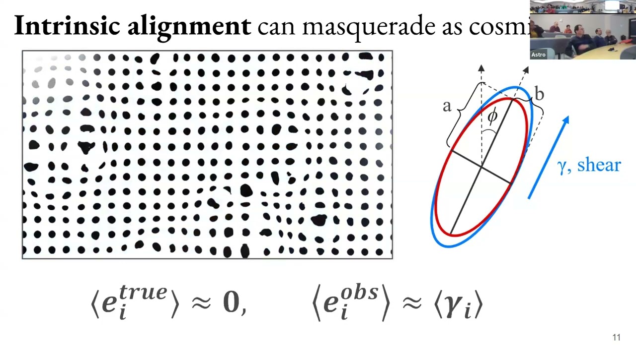
[00:00:20]We we um talked about the lensing distortion tensor and what that does to uh images of galaxies and or anything else. Um and so I wanted to start um getting into the weeds of cosmic shear where cosmic shear when we saw shear was one of the components of the distortion tensor that just changes the shapes of the of whatever images you're looking at. Uh cosmic shear is also the name that we give to just the the idea of getting lensing from the shapes of galaxies. Right? So this whenever you hear cosmic shear just think of um weak galaxy lensing right where the source is a galaxy um um all right so how does that work um so what do we measure what we measure is for a given galaxy we will measure its observed elipicity and what we said is that that is the um true electricity which I'm going to write as EI N. Remember I is either one or two because there's two components to the electricity.

[00:01:29]And so this would be the true unlensed electricity of the galaxy plus a contribution coming from weak lensing which is just the sheer component of the of the distortion tensor. Okay.

[00:01:42]Um so this is the intrinsic galaxy shape as you measure it where in practice we will see that what you measure is not just the intrinsic galaxy shape plus lensing but also any any source source of noise in the measurement of that shape but just think of this as the true unlensed um shape for now. Um so in practice what does that look uh look like right this let's imagine that you've observed um a pixel in the sky. So this is just some tiny region in the sky where you have a bunch of galaxies and for each galaxy you may have uh uh at the position of each galaxy you may have the corresponding value for the sheer field um right which I'm going to write as a rod um meaning an electricity pointing in a particular direction right so let's say this is the the shear component and the shear component will be correlated across this pixel because it's all caused by the same intervening large scale structure over here and you're observing from over there, right?

[00:02:40]Um, but what you observe is not just this. It's this plus the the intrinsic shape. And so the question is in the same pixel, how different the the intrinsic shapes are from the from the cosmic shear. And it turns out that cosmic shear compared to the typical electricity of a galaxy is a very tiny component. So the typical shape of a galaxy will be actually the typical electricity will be quite large compared to the cosmic shear. Right? And for each of these galaxies, you'll have a different ellipticity that is much larger than the um than the sheer component. Okay.

[00:03:18]Um um and it's the sum of these two that will give you the the actual the actual measured value for the for the for the thing that you that you're actually measuring, right? Um so what you do is um the main assumption is that the shapes the intrinsic shapes of galaxies are uncorrelated right so the shape of a galaxy here here and here they have nothing to do with one another uh and the only thing that will correlate them is the cosmic shear so what you do is you say okay I don't care I'm going to try to average down this noise by just taking an average over all these galaxies and just getting a single measurement of the of the shear effect um at the center of this pixel let's And um and the hope is that you have a large enough number density of galaxies that you can average down this noise, right? And get a measurement of the average shear within within that region.

[00:04:12]Um so that's kind of the idea and we'll see how problematic these these intrinsic shapes are uh later on. But for now, let's imagine that we can do this, right? We can make a map of the of the cosmic shear for all the galaxies in our in our survey. Um we said because it's a bit annoying to have to deal with two components of the of the cosmic shear. Um cosmic shear comes from the same single scalar quantity as as for example the the lensing convergence which is the lensing potential right. Um and so let's think of of the lensing potential sorry the the lensing convergence itself. Let's imagine that instead of measuring shear what we're measuring is actually the convergence.

[00:04:52]This is just because it's going to make the math a bit easier. Um but the you know none of the conclusions and kind of ideas that we're going to uh show here actually change that much. Um maybe in the last lecture we can introduce some of the subtleties of of going from shear to to convergence. But but for now let's imagine that we can actually just measure this directly from from these observations. We can transform basically our measurements of of gamma into kapa.

[00:05:16]And that's actually true. Okay. Well, let's take a simplified um picture in which all of our galaxies are sitting at the same distance from us, right? So, this is the distance to the source is the same for all our galaxies. Um and then in in that case, we worked out yesterday where the corresponding convergence would be, right? It's just given by this integral along the line of sight of the uh matter density fluctuations times this cont this kind of um radial function here um which came from the lensing equation.

[00:05:49]All right. But that's not actually how um reality works, right? We don't have all galaxies lying at the same red shift. Usually what we have um is uh as a function of red shift, you have uh galaxies lying in some kind of um range of red shifts, right? So some kind of bin of red shifts with a given red shift distribution. Let's say this is P of zed. um um meaning the the distribution of red shifts of your of your galaxies.

[00:06:21]Um all right, but then that doesn't change things too much, right? So the um the the kappa field that you would measure from all of these galaxies. Now it wouldn't be the kappa at the particular red shift, but the average of all the kapas at different red shifts.

[00:06:36]Right? So this would be just an integral over all possible red shifts of um the p of zed times the kapa at that particular direction in the sky for sources at a red shift zed. Okay. So it's basically this um for sources at a given distance. Right?

[00:06:58]So that's the thing that I'm inserting in that in that other equation. Right?

[00:07:02]So if we if we do that what do we get?

[00:07:04]We get 3 /2 h^ 2 omega m time an integral from 0 um to infinity dz p of zed times an integral d kai from 0 to k of zed um of uh k / the scale factor at that value of k times k of zed minus k / k of zed and then times delta of k n z of k. All right.

[00:07:43]So in principle that would be it. That's the quantity we're calculating. Does that make sense so far?

[00:07:51]Um the problem with this expression is that if we want to eventually make a theoretical prediction for this, it's kind of annoying because the quantity we care about this one is embedded in two different integrals. And that's a bit annoying. Um so instead what we can do is change the order of integration.

[00:08:09]And this is something that you learned to do in the first year of maths if not earlier. So I'll let you do that yourselves as a as a problem.

[00:08:18]Uh so if you change that order of integration you get an simpler integral um which look like looks like this. So it's an integral along the line of sight um of a radial kernel that I'm going to call the lensing kernel uh times the density uh the over density field kapa n comma z of kai.

[00:08:44]Okay. And this lensing kernel is something that you can just compute um externally. QL of K is uh 3 /2 H^ 2 omega M* K / A of K and then the integral uh from zed for that K to infinity D z prime P of Z prime and then I'm going to go into the board 1 minus k / k of z uh prime.

[00:09:32]Um so that like looks like a complicated equation but we can actually we can actually make sense of it. Um so at a given distance sky this lensing kernel is the integral of the p of zed times some function. the p of zed uh integrated from the red shift corresponding to this distance all the way to infinity. Right? So that means if we were here for example, let's say we're here, that lensing kernel should be what?

[00:10:07]Zero. Yeah, zero. Because you know p of zed at all those red chips is just zero.

[00:10:12]It's beyond uh we're beyond the p of zed, right? So here it would be 0 0. So it will be zero up until the point where we get to uh p of zed right um and then it will start picking up um and then eventually die down like that.

[00:10:27]Um right um so this is the the shape it has right it's very similar to the shape that this function itself has this one here um and that's um you know if you plot this this is a second order polomial in kai uh so it's basically a parabola that looks like this from the sources so this is the position of the source um to to zero uh it's basically a parabola that's what this what this kernel does this is essentially ly the same except now your sources are a bit diffused. They're not exactly at the same red shift. So at the beginning it won't be exactly a parabola. It will it will basically follow the red distribution but then then keep going like a parabola all the way to um to redie zero. Um so this is this is the Q this is QL right ql of zed let's say. Um and then we can wonder does that make sense right that means that kappa is receives contribution contributions from all red shifts from the red shift of the sources to zero right does that make sense so it's affected by the large scale structure all the way along the line of sight that's what you would expect right that's what lensing does lensing will deflect photons um through all of the large scale structure from the sources all the way to to you right so that's why the the lensing kernel has this shape. It basically tells you about the contribution from different um points along the photo trajectory um is right.

[00:11:59]Okay. And this will be quite important actually to understand why weak lensing is so sensitive to small scale structure. So we'll come back to this picture uh later on.

[00:12:10]um P of Z P will depend on the sample of galaxies that you have and how you've selected that that sample, right? So if you have sufficiently good red shift measurements for your galaxies, you'll be able to select galaxies in a particular range of of red shifts. So that means that you can isolate them to live in a particular region in in red shift. If you have really poor red shift measurements for your galaxies, it will be difficult for you to locate them in a in a given region of space. So you might have to you might have a very broad retribution uh and you need to worry about how you estimate that retribution but uh we'll talk about that actually tomorrow but yeah P of Z yeah the assumption is that you um the assumption here at least is that um whatever sample of galaxies you you've selected um uh they've been selected in roughly the same way across the sky so they have the same retribution across the sky. Yeah. Um there's um obviously this is something you one should worry about, right? So if if uh the galaxies you're using are if the sample you're using is significantly fainter in a given region in space than other, you could imagine that the sample is actually different. So your red distribution actually varies across the sky. Um and you're not really sampling the same red shifts in this region or in this region. So then the total kappa field the average kappa field actually receives an extra contribution coming from spatial variations in the in the p of zed. Um um and those can be relevant. They if you have significant inhomogeneity in your survey it can actually be be relevant. Um yeah other questions?

[00:13:53]No.

[00:13:55]Okay.

[00:13:57]Um so now we are working this is the the first instance of of a field uh that is a projected field right and now we have a quantity that's defined on the sphere the same way that that manu yesterday was talking about the temperature fluctuations of the CMBB this is a field now that is defined on the sphere and uh in the first lecture we saw how we deal with uh stoastic fields that are defined in three dimensions now we have to deal with with the two dimensional ones it's good that um that Manu kind of did half of the work for me. Um uh so I wanted to take just a little bit of time about talk uh to talk about stoastic fields uh in on the sphere right um in S2.

[00:14:45]Um um so um I'm going to skip a lot of the stuff that I had written here because actually Manu talked about a lot of this. Uh but the idea now is the same treatment that we had for um for you know uh fields defined in three dimensions. Now we think we need to think about fields defined on the sphere.

[00:15:06]Um so you know we talked about stoastic fields in 3D just thinking of them as um uh you know vectors of multiple random variables characterized by a given multivaried distribution of them. This is exactly the same idea except these points are not the points within a sphere. So nothing changes in in that picture.

[00:15:24]Um you can still think about statistical isotropy right the idea that the sky should be the same no matter where you look at but also in which orientation you look at the sky. So whether I tilt my head like this or not um and that will involve that that will imply certain things about the um about this right. So for example, what would the so the twopoint function between two fields defined on the sphere at positions uh n1 and n_sub_2 b n2 right? If we have statistical isotropy this two point function should only depend on what?

[00:16:03]Yeah, the relative angle between the two points, right? And that's given by the so this should be some function that only depends on essentially the cosine of the angle between the two vectors. So n1 n2 basically so that's the only way that things should depend. So this is what you would call the correlation function AB. All right. And um right one another thing that we saw was a nice thing to do for um for fields defined in 3D is to take their for transform right uh for fields um defined on the sphere.

[00:16:38]Manual already told us the the sensible transformation to do here is the spherical harmonic transform. Um so uh we define the spherical harmonic coefficients alm as being the integral uh over the whole sphere of a of n times the spherical harmonic coefficient yl of n complex conjugate. Um and then the the inverse transform is just basically the expansion of um your uh uh field into spherical harmonics. So sum over all the l's from 0 to infinity sum over m from minus l to l. You've seen all of that in in quantum mechanics if not in in many other areas of uh ALM times YM.

[00:17:28]Okay, it's kind of the analogous of of a um for a transform and an an inverse for a transform and um Manu yesterday introduced this in the flat sky approximation where you can actually replace replace this by for transforms and inverse for transforms in 2D. Um and what I would say is the main thing to bear in mind is that this is you can think of a spherical harmonic transform in almost exactly the same terms as what you would think of uh for a transform.

[00:17:56]you can identify L as the modulus of a wave vector in in 3D or in 2D in this case, right? So just think of it as essentially a a wave vector meaning um an inverse wavelength but now these are wavelengths defined under fear. So they're angular wavelengths I guess. Um and uh yeah so so angular separations corresponding to a uh so typical kind of let's say yeah wavelength on the sky uh associated with a given L. Um Mano had a 2 pi. I like to think of pi instead but it doesn't really matter. It's on an order of magnitude right. Um so that's how you relate an L to a given typical angular separation or angular scale that the that the spherical harmonic is is probing. Um okay.

[00:18:46]Um all right. And so uh the same way that we have um a consequence for statistical isotropy and homogeneity in the 3D case, we have another similar consequence in in terms of um of this the spherical harmonics um of of fields in 2D which is how we define the angular power spectrum. So the idea is that if you have statistical isotropy and you look at the correlator between ALM and B L prime M prime complex conjugate um this has to be proportional to the chronicer delta L L prime and MM prime. So um different harmonic coefficients should be uncorrelated to one another if you have statistical isotropy. And the proportionality constant is what we call the power spectrum CL ab uh which only depends on the modulus of the of the um of the wave vector meaning the the the L um harmonic number.

[00:19:59]All right. So this is all stuff that Manu talked about um yesterday I think.

[00:20:05]Any questions about any of this interpretation of this or anything? No.

[00:20:10]Um what's interesting I think is how we connect uh this angular power spectra which are the things that we're going to be able to calculate for for things like the convergence field how we relate that with the with the physical quantities that we care about which are things like the over density uh matter over density right um so in general uh let's think of a projected field like this afn which can always or often it can be written as an as a line of sight integral of some threedimensional field, right? So, uh we can always write this as some kind of integral along the line of sight of a kernel associated with with that quantity times a 3D quantity. So, something defined in in three dimensions um evaluated along the light cone uh like that.

[00:21:01]Okay.

[00:21:04]Um so this is what we can observe. This is what we would like to observe, right?

[00:21:09]or what we would like to have access to.

[00:21:11]So the question is how do we relate the statistics of this field to the statistic of that other field and in particular we care about the angular power spectrum. So let's say we're looking at the angular power spectrum between field A and field B.

[00:21:25]Um so the relation between this angular power spectrum and the corresponding 3D power spectrum of the 3D quantities is given through something that we call the limber equation.

[00:21:40]um which is given by an integral along the line of sight uh divided by k^ squ uh then the radial kernels of the two quantities that you're correlating qa of kai qb of kai times the 3D power spectrum of the corresponding 3D quantities. So I'm going to write that as P A B of K and uh zed.

[00:22:10]And uh and then the question is what what's the 3D um wave number? How does it relate to the 2D um wave number or the 2D multiple? Um and that's through uh the relation that you saw yesterday from Manus U slides. Um so K can be related to an so a 3D wave number can be related to a to a 2D one uh by simply dividing by the moving distance to to the quantity that you're that you're looking at right a more accurate version of this is that this should be L plus one half but you know this 1/2 doesn't really matter if you're at sufficiently high L which will be the case for for the most part um this is the limber equation I'm not I haven't derived this at all right so if you want to look at the derivation of this I can give you references for And in fact this limber equation is um is an approximation right so it's not this actually is an approximation the the exact equation is a bit more it's a bit longer it involves bessel functions that complicate the its expression a little bit so um and I'm not going to I don't think it's worth the time to discuss that in much detail for most of what we're going to discuss this is limar is is an appropriate approximation um [Music] cases in which you will have to worry that limber is not um is not good enough is when the width of these radial kernels.

[00:23:41]So let's say that you have a radial kernel like that and the typical width of this radial kernel if that width is comparable to the typical correlation length of the quantities that you're correlating. Right? So if we're thinking about the matter distribution, we saw, you know, the matter correlation function kind of dies down at separations of a few mega parc.

[00:24:01]Um, so if you have a kernel that has a width of a few tens of mega parex or smaller, then limber is going to fail miserably. So this is will be a very bad approximation. For the most part, we have kernels that span several hundreds of mega parex where the correlation function is essentially zero or very very small. So limber is a good approximation for most of the observables that we're going to look at.

[00:24:21]Okay. So that's why I don't want to go into the details of the non- limber stuff. Um um and also you know limber limber is really useful because it will give us intuition about which scales uh which physical scales are actually contributing to the different observables that we that we will look at and we'll we'll talk about that later on.

[00:24:43]Did that make sense? Any questions so far? Okay.

[00:24:59]>> Yep.

[00:25:06]>> Yep. Yes, that's right. Yeah. Yeah.

[00:25:09]Yeah.

[00:25:10]Uh the question was just to make sure I guess that um if your red shift bins are really really tiny right so if you progressively make them smaller then limber will start failing and the answer is yes you should worry about you know typical red shift bin you know delta zed of about 0.01 01 I think that's about 30 megap sec uh that's definitely going to start failing uh limber approximation right so um whereas if you have bins of 01 0.1 it's probably fine u yeah um and it will so limber uh will start failing at the lowest multiples first and then it will progressively go to the to the higher ones so even you can probably get away with limber if you're really interested in the smallest um scales right the the the large the largest multiple so it will start failing I'm not sure what I said before it will start failing on large scales, meaning the smallest multiples and then but if you're interesting in small scales, this you know you can you can probably get away with it with with limber u often.

[00:26:04]Um um yeah. Okay.

[00:26:12]Um great.

[00:26:16]Okay. So um so then uh how do we usually uh extract information from week lensing? Usually what we will do is we will have um we will have uh I'm going to use a different color for this. We will have uh samples of galaxies that we've selected at different red shifts. So we'll have what we call tomographic bins of of galaxies, right? Um and we'll have made maps of the kappa fields for each of them and then we'll be able to look at auto and crossorrelations of all those um of all those quantities. So the the actual observable we tend to look at is the um is the angular power spectrum the kappa field um and another capa field at two different red shift bins let's call them i and j um so this is bin i bin j for example um so using the limber equation this is just an integral along the line of sight d kai over kai squ uh the lensing kernel for bin i of kai the lensing kernel uh for bin J of Kai 10 times the power spectrum of the threedimensional field that lensing maps which is the matter over density. So this will be then the matter power spectrum. I'm going to call that PMM of uh L over Kai and red shift implicitly. Red shift is the red shift corresponding to to Kai. Okay.

[00:27:43]um for reasons that have to do with mostly sociological tradition and uh and and how the field has evolved uh in large scale structure a lot of the early analysis and even currently I think uh I would say about 60% or so of all we lensing analysis don't really use a power spectrum but use the corresponding version of the correlation function. Um we saw that in 3D there's a relationship actually between power spectra and correlation function. So let me write that here for 2D in case you want to look at that. Um so the the correlation function um at an given angular separation theta is sum over all the uh multiples L 2 L + 1 / 4 pi times the legendary polomial um evaluated at cosine of theta times the CL. Okay, so that's how you relate one with the other. Remember in in in 2D sorry in in 3D you had a for transform relating correlation function and uh CL's in in on the sky you have a a transform in terms of legendary polomials. Okay. Um all right. Anyway, so um often you'll see cosmicure analysis being done in terms of correlation functions and I just want to I just want to maybe we're going to keep talking about kappa uh because I'm a power spectrum person. So I like to think about it in this case but so that if you read the paper you kind of know what they're talking about. Um I wanted to kind of clarify the usual notation that is used in those papers. Um so let's say that you have two galaxies right here and here and you're now what you care about is correlating the value of the cosmic sheare in these two galaxies. Um right uh but then you need to worry about how you define the cosmic shear field itself. Um is there a pointer somewhere? Yes. Um right so you have this galaxy and this other galaxy here. Um and so the the question is um what's the natural set of coordinates that I should use to define the elicities of these galaxies right so um if you have two galaxies the natural um the the the line that separates the two galaxies that gives you a clear preferred orientation with which to um to define your your coordinates. Right?

[00:30:04]So a natural set of coordinates would be to put one of your axis along this direction and the other one being the perpendicular axis. Okay. Um in often the ellipticities that you get for a given galaxy they will not be given in this coordinates. They'll be given in in in sky coordinates meaning x will be usually x is right ascension and sorry no x is declination and y is right right ascension usually. Um uh so you need to rotate the value of the ellipticities or or shear that you get usually from in sky coordinates rotate them to the to the kind of pair-wise coordinate um um coordinate system right um so that's you know this is the transformation essentially that you would need to do to go from gamma 1 gamma 2 which are the which are the field the the the sheer uh or electricity measurements in sky coordinates to what's called gamma t and gamma x which are or gamma cross which are uh essentially versions of gamma 1 and gamma 2 in these new coordinates. Um and here's the idea right so if you have a galaxy or uh a galaxy for which gamma t is negative that means that it's elliptricities um along the line of sight uh from sorry along the line that connects it to another galaxy right that's a negative gamma t a positive gamma t is when it's uh tangentially oriented remember that um lensing causes um this tangential orientation so it makes sense that with this definition positive gamma t should correspond to um to tangentially oriented things. Then gamma cross um being uh uh positive or negative uh corresponds to ellipticities that are oriented about 45° with respect to this this direction here. And why 45 instead of 90 has to do with the fact that um that cosmic shear is a spin two field. So it's basically for a given galaxy, it's a rod rather than an arrow with a particular direction. Uh so you can rotate this rod by uh 180 degrees and get the same rod again. Um anyway that's subtleties that I didn't want to get into. If you um if you look at um many cosmic sheer analysis things will be expressed in terms of gamma t and gamma x and then what you care about is the correlations between gamma t and gamma x in two different galaxies.

[00:32:25]Right? Um and that gives rise to two different correlation functions.

[00:32:31]What's commonly called G uh plus or minus and these are just the correlators of different combinations of gamma t and gamma x. So in particular these are the correlators that you would look at. It's gamma t um at n1 with gamma t at n2. And the logic is that n1 and n2 are separated by an angle theta plus or minus um gamma x at n1 and gamma uh x uh at n2.

[00:33:09]These are the two different correlators that people usually um look at.

[00:33:15]Um, you might wonder how you could phrase this in terms of the convergence power spectrum because that's what we're going to be talking about. And there's actually a relatively simple relation between the two of them.

[00:33:28]Uh so it's an integral um over all possible multiples dl * l / 4 pi 2 pi um the bessel function uh often called the cylindrical bessel function of order 2 plus or minus 2 sorry minus plus - + 2 of l * theta times the capa kapa power spectum Okay, so if you ever see or have to analyze data in in the form of correlation functions, you can still just compute your power spectra and in fact that's usually the first step and then translate them into correlation functions just using this this expression here.

[00:34:16]Um this expression is actually a kind of flat sky approximation version of this other expression in terms of legendary polinomials. So they're actually equivalent. Um yeah.

[00:34:31]All right.

[00:34:32]Just wanted to dispel this because actually you'll see lots of papers that use this kind of notation. Uh more and more people now are are actually using power spectra to analyze cosmic shear data. So we'll continue uh working with that.

[00:34:45]Does that make sense? Questions? Yeah.

[00:34:49]Say again. No cross term. Um so there is a cross term and that would give you another type of correlation function for cosmic shear you would expect that to be exactly zero. So you can measure that correlation function as a null test. So if that thing is not zero that probably means that you have systematics in your in your data. Um yeah we'll talk a little bit more about that because that's one of the diagnostics that you can do to to see if you have problems in your data. Um, yeah.

[00:35:22]Yeah.

[00:35:27]Where does it come from?

[00:35:29]Why in particular look at this plus or minus that? Yeah. So, um, the idea is that as far as I understand, I need to remind myself of this. um you look at this particular combinations um I think it's because uh those particular combinations will be uh cord it um they will not depend on the particular coordinates that you've chosen I think I'm not completely sure actually um I'm not a fan of real space analysis um but I think that's the reason for for that um but other than that just chalk it up to tradition and this is what people have been doing for a long time basically Okay. Yeah. Um >> uh no. So, so you will need to define them for each pair of points in your survey, right? So, you would go over each pair of galaxies in your survey.

[00:36:28]For each pair, you would define the preferred coordinates like that. And then you would redefine the values of gamma t and gamma x for for each of the two uh galaxies along this this preferred axis.

[00:36:40]Compute this and then um compute these products, right? And then do this for all pairs of galaxies and then average over pairs of galaxies. That's how you would Yeah. Yes. Exactly. Yes. Yeah. Yeah.

[00:36:54]Yeah. Yeah. This is supposed to be observer here and this is N1 N2 basically.

[00:37:04]Yeah.

[00:37:08]Yeah.

[00:37:12]Uh great.

[00:37:15]Okay. Um so next I uh we're going to keep talking about things in terms of a of Angular power spectra. um uh but I wanted to mention this. So let's let's get back to to power spectra and uh let's start thinking about the main um challenges that we have with cosmic shear. What are the main problems that cosmic shear needs to needs to look at um or needs to be worried about.

[00:37:41]So um first of all as we said uh what we measure is actually a noise dominated signal or or quantity right we said that for any any given galaxy the contribution from lensing to its electricity is usually much smaller than the raw electricity itself of the galaxy and that's why we need lots of galaxies to average average that down. Um let's imagine that we had no lensing, right?

[00:38:07]So we had uh our measurements of the electricities were literally just the uncorrelated um uh electricities of the of the different galaxies.

[00:38:18]Um that would mean effectively if we're thinking of this in terms of kappa, a measurement of kapa at each electricity at each galaxy, that would mean we're measuring a value of kappa that is essentially uncorrelated across different different galaxies. If I had to plot the the CL capaca in that case, um what do you think that would look like? So that means the power spectrum of a signal that is completely uncorrelated across different points in the sky.

[00:38:56]Someone said zero. It's not zero.

[00:39:00]flat. Why flat? So that's the the right answer is that it would be flat. So anything that is completely uncorrelated across different points in the in the sky would be flat. But why should it be flat?

[00:39:15]We can um maybe remember in 3D there was a very simple relationship between a power spectrum and a correlation function, right? Um so a power spectrum would be the inverse for a transform of a correlation function, right? So it's something like u it's proportional to an integral over all positions in space um of a correlation function uh as a function of of that right of x. Um so what does the correlation function of an uncorrelated uh field look like?

[00:39:54]Sorry, >> what did you say?

[00:40:00]>> I think it makes sense. It should be zero. So if you're correlating a value of the field here and here, it should be zero. But if you're correlating a value of the field here and here, that should be something, right? Because the the the field itself will have some local variance, but not but it will be uncorrelated across different. So that means that this should be proportional to uh direct delta right um at x equals z basically right so that uh sorry and this was this e to the i kx I forgot about the the vital part um okay but if this is just gets contribution from x equals z then this is equal to one so you get something that doesn't depend on k right the only dependence on k is here and the only contribution comes from x equals zero so the right so that's the way to see it I guess a power spectrum for an uncorrelated field is just a constant and that uh also extends to the 2D version of this. It's just that it's a bit easier to think of it this in terms of for transforms. Um okay so if we have um white noise this is what we call a white noise component something that is uncorrelated across different points in the sky. So if we have a white noise component it will look like uh like a constant right in reality we said our measurements are not just the the noise like shapes but also the the contribution from weak lensing to each of those shapes.

[00:41:15]Um, and we haven't actually haven't shown you this yet, right? But we can think about what the power spectrum of this this thing would be, right? It's uh it's something that needs to look like this.

[00:41:28]Uh where this is the matter power spectrum. We'll see later on that that leads to a shape that kind of looks like the matter power spectrum, meaning something that decays at high values of L and then maybe might have some turnaround here. Um, right. So it usually looks something like this. Um so this is the this is the gamma part or the kapa part. So this is the signal and this is the noise component.

[00:41:56]Um and so what that means is that for cosmic here but this is actually something that happens for any measurements you'll have a regime of scales where your measurements are dominated by the signal itself. That means that the the your measurement errors will be dominated by the uncertainty in the signal. This is what um what uh Manu called the cosmic variance um source of the noise of the of the measurement errors. Um and then there will be other scales where you're dominated by noise. Um okay.

[00:42:32]And there's nothing you can do to reduce these errors when you're signal dominated. But there's definitely things you can do to um to uh to reduce errors in the noiseated regime. Basically, you want to lower this noise level as much as possible. Right? So, how do you think we can uh reduce the noise level for cosmic shear? What can we do about a um a survey of galaxies in order to reduce that? um get more galaxies indeed. Yes. Uh so this noise power spectrum let's call it CLN for noise um is basically it has two components right. So if we could measure the ellipticities really really well that should lower the noise but also if we have more galaxies we can average over more galaxies and and get lower noise right so it has two components. So it's proportional to the error with which we can measure electricities squared. So this is the the typical um scatter of elicities um uh divided by the number the angular number density in ster radians inverse ster radiandians of of galaxies in your survey. So if you have more galaxies you lower the noise.

[00:43:38]If you have smaller measurement errors then you also lower the the noise. Okay.

[00:43:43]And so you bring this down. Um the first measurements of weak lensing were in this regime where the noise was up here was actually much higher than the signal. So you um you could maybe see the signal on the largest scales after um um um you know after measuring the power spectrum but it was completely noise dominated. The error bars are completely noise dominated for something like LSST you expect to be in this regime um where this L here will be of the order of a few hundred um basically let's say order 200 or something like that. It probably depends on on the settings that you're looking at. Um so that you know L of 200 uh remember the corresponding angle angular scale is uh pi over L so pi over 200 this would be in radians if we do it in degrees this would be about 180 over 200 so that's about one degree okay so that means that even LSST so which is one of the um one of the newest uh and most advanced surveys things will still for cosmic share will still uh noise dominated on relatively small scales. That doesn't mean that we can't measure the small scales. It's just that the error bars in our measurements will be dominated by noise rather than by than signal, right? Um so this is I think one of the most the most important drawbacks of cosmic shear is that you're it's very difficult to not be noise dominated. It just there's a lot of noise. So you just need to accumulate as many galaxies as possible. Um um and one just to give you an idea of how that has evolved over time. This is a picture of of different galaxy surveys. Thanks a lot. Uh um as a function of two of the main variables that we care about. So it's on the x-axis you have the volume of space that they cover. So the larger the volume the the better your power spectrum measurements will be. Um but also the source density, right? So that tells you how many how many sources you uh you have to average down the noise.

[00:45:44]Um and so um the stage three surveys currently the the ones that that we currently have um DES kits some of you might be involved in those. They're in this regime. Fairly large volumes um but still you know relatively low number densities. When we say low number densities they're actually quite high number densities.

[00:46:05]This is 10 galaxies per square arc minute. An arc minute is very small and you have 10 galaxies per per square ar minute in those cases. Um um so you know you're you're talking about of the order of a billion galaxies in the case of DS or something like that. Um and we want to move to this other regime right LSST Uklid potentially the Roman space telescope uh where where you know the typical source density is about three to four times larger and you cover a much larger uh portion of the sky. Um that will as I said this will lower the noise but it will not bring you to the level where everything is signal dominated. uh you would still have to deal with with quite a lot of noise. Um okay. Yep.

[00:46:57]>> Yeah. I think I think it probably depends on what was assumed. I think this probably is I I I would need to check how this um how this figure was generated. This is in the in the wig lensing review that I recommend you look at if you're interested in wig lensing from this year. Um my guess is that this corresponds to the target depth of LSST.

[00:47:20]This might be the actually realized depth of HSC meaning the the depth that they could use for their weak lensing analysis which is always lower than you would think right so you might think that you can go to magnitude 27 or something like that. In reality, HSC uses magnitude 24.5 or something. So that means significantly lower number density. That's my guess. But but it's true that HSC was supposed to be almost as as deep as LSST. So yeah. Um so it might be that in the end we're we're in this regime instead instead of that regime, right? So it will depend on on the cuts that we need to do on the real data to to get it to that level. Um yeah, but that's a very very good question. Um okay. Um so that's challenge number one is we need to deal with a lot of noise. Uh challenge number two which uh was uh asked about a couple of times already is um we've been saying that this noise component here is flat. It's completely uncorrelated. So you know we just need to estimate it this way and subtract it from our measurements and we're done with it. Um by the way I didn't say the the intrinsic ellipticity of galaxies is of the order of 0 point. So the scattering that elliptic is 0.27 or so, right? Um whereas the cosmic shear component is percent level. Um yeah, so that's why it dominates so much. Um anyway, uh but we said what if these shapes are actually correlated with one another, right?

[00:48:47]Couldn't couldn't it be that the actually intrinsic shape of the galaxies are correlated? You could imagine that there might be some physical processes that align galaxies that are nearby with one another, right? Um so that's what we that's the other challenge one one of the other challenges that a cosmic here needs to deal with which is intrinsic alignments.

[00:49:04]That means the the fact that the intrinsic shapes of galaxies might actually be correlated with one another.

[00:49:18]Ah I didn't that's okay. Um um right so let's split EN so the the intrinsic uh measurement sorry the intrinsic electricity of of a given galaxy into two components one of them which is correlated um with the large scale structure I'm going to call that EI for intrinsic um and then I'm going to call the remainder I'm just going to call it noise n so the you know the the component of the electricity that doesn't really correlate across different uh galaxies. Um and so what physical processes could uh lead to a correlation between the shapes of galaxies that are close to one another. All right? Or the correlation of the elicities of galaxies with the large scale structure. Okay?

[00:50:11]And so the simplest model that can give us that is something called tidal alignment.

[00:50:23]And it's it's a physical process that is actually quite quite easy to understand, right? So let's imagine that we have a large structure here.

[00:50:31]So something massive and then we have a galaxy nearby. Let's say here. Let's say that this galaxy was originally a sphere. Um just because we like to do that in physics. Um um so galaxies are extended objects. Um and we need we we can think about how the gravity of this object here would affect the the shape of of this galaxy, this blob of of stars, right? And so let's think of the different gravitational forces that are acting on this on this galaxy. So right there will be gravitational attraction acting on this point in the galaxy. Some some gravitational force in that direction.

[00:51:09]Uh also on this other end of the galaxy, right?

[00:51:14]Uh but that uh right uh so that that'll be that'll be something that happens right uh there will also be a gradational force in this direction and a gravitational force in that direction right um so let me zoom zoom into this thing so now let's zoom into the galaxy I'm going to draw it like this so we're saying graational forces for example here and here.

[00:51:43]Um but this gravitational forces should be slightly different, right? Um this it should be a bit weaker farther away than closer to the to the object. So overall that means that well this might move the galaxy closer but in terms of its shape what this will do is basically elongate it in this direction, right? Because because it will have a differential force that that uh kind of elongates it in that direction. Then the other in the transverse directions we said if we're kind of close to this object you'll have a force that points like that in this direction and a force that points like that in this direction. Uh and there will be a a perpendicular component of this force that tends to squash the galaxy in this direction. Right? So these tidal tidal forces meaning the the differential forces across the this extended object what they will do to this galaxy is to make it look elongated in this direction right it will squash it in this direction and it will stretch it in the in the opposite direction.

[00:52:40]Um and this is very different from weak lensing right there's no weak lensing going on here. This is just the local gravitational field uh um around this object. Okay. And how much this galaxy gets stretched depends on the on on the on the internal kind of uh structure of this galaxy. How strong the internal gravitational pull of the bulge of the galaxy etc. um uh the the kind of the you know the the radial motions of the stars within it whether they can resist this these tidal forces etc. So so it's not so you can expect this kind of effect but it's clear it's not obvious to know how uh large the effect will be right.

[00:53:19]So the the usual idea is to um is to say okay the uh remember we we were talking about the inertia tensor of of the shape of a given galaxy. Um so we think uh within this this title alignment model we say okay we the the intrinsic contribution to the to the inertia tensor of of a galaxy should be proportional to this uh to this effect right proportional to the differential in the forces of um of gravity across the these objects right forces of gravity that means the gradient of the gravitational potential and we're now looking at the differential of that across the surface this uh source the the the extent of the galaxy. So that means second derivatives of the gravitational potential right? Uh so we say that this should be proportional to the second derivatives of the gravitational potential itself.

[00:54:15]Okay. And this is the local gravitational potential at the red shift of these of these galaxies. Right?

[00:54:21]So this is the title alignment model.

[00:54:22]the title title alignment model what what it says is that the the alignment the the um the shapes of galaxies might receive an additional contribution from the local title gravitational forces and we don't know what the proportionality factor is here right in weak lensing we know what the proportionality factor is remember for weak lensing we were saying that qig um was equal to second derivatives dj of the of the not the graational potential but the lensing potential right which is an integrated quantity not the local one. Um for intrinsic ones it's the local gravitational potential but actually we don't know the proportionality uh constant here.

[00:55:03]Questions this was remember from yesterday I'm using too many Q's I think in my in my notation. uh qi j was the integral over your image of delta theta i delta theta j times the intensity uh sorry the intensity of your image right um theta right the inertia tensor of of uh of your galaxy yeah so it's basically the quantity that we use to describe the shape of of our galaxy yeah Okay.

[00:55:50]>> Say that again. What's the >> um well the the source meaning the physical origin of this effect is the gravitational force itself. What kinds of sources are more affected by this? Um the theory or the kind of expect well what we have measured so far is that the only types of galaxies that seem to have uh this type of alignment uh or that we see are aligned are um elliptical galaxies which mostly means well almost mostly means red galaxies.

[00:56:28]Um so early type galaxies these are galaxies that don't have a you know they're not spirals so they're they don't have a clear um plane of angular momentum um where you have coherent motions like that uh but you have just random motions in kind of a blob of stars basically and I could imagine why that but there's probably several reasons why that those might align more.

[00:56:47]One of them is if you have a blob of stars maybe it's easier to deform it uh rather than have something with a coherent kind of motion. And the other one is um uh elliptical galaxies. The theory is that they probably form after merger or of different uh galaxies. And those mergers usually happen along the lines of gravitational forces. Right? So you could imagine that after a merger whatever happens afterwards might be aligned with those with those forces.

[00:57:13]>> Anything anything that causes uh gravity, right? So this whatever what it could be just dark matter halo or of something or something like that, right?

[00:57:21]Um yeah.

[00:57:23]Um yeah for this yeah so the I mean just imagine what what should happen to the earth right as it as it rotates around the sun um I'll just repeat that. So, so imagine this is the sun and this is the earth. The earth is a finite planet, right? Um, if you look at the graational forces uh on the earth, right? There should be a graational force on this side of the earth and on the other side, but this one should be a bit weaker, right? Um, so that means that you know the the shape of the earth should have uh should have a a shearing force in this direction that kind of stretches it, right?

[00:58:07]um and tidal forces in that direction and that direction because they they will have a you know they'll be pointing in that direction but that means that they have a a component in the perpendicular direction that will tend to squash the earth in the in the the other direction right um so you you expect title alignments to squash galaxies in in that direction yeah say again Why this? Because what what right? So what are the forces? What's the origin of this squashing? It's the difference in the force at this point and at this point, right? So it's like force at some point in your object minus force at some point plus the extent of your object, right? Um and this is just the gradient of the gravitational potential um at some point in your object minus the gradient in the gravitational potential at another point x plus l in your in your object. So this is looks like a second derivative right of your gravitational potential already. Um yeah.

[00:59:17]Yeah.

[00:59:28]This is the second moment.

[00:59:30]Yes.

[00:59:32]Yeah.

[00:59:34]Um Okay.

[00:59:37]Uh but okay. What should we expect intrinsic alignments to do to our signal? Remember we said if we had a massive structure somewhere along the line of sight of our from our sources that weak lensing will tend to generate tang tangential um alignment of the of the galaxies.

[00:59:57]Right? So this is the effect from weak lensing for any source sorry any lens along the line of sight. If this lens happens to be close to these galaxies, then you'll also have uh a title alignment effect and that title alignment we said should align galaxies in that in the opposite direction.

[01:00:19]Um so this is this is lensing and this is intrinsic alignments.

[01:00:25]Uh so intrinsic alignments overall they will decrease the lensing signal um by some amount.

[01:00:32]Luckily for us, intrinsic alignments are is a relatively small effect. Right?

[01:00:36]Most of our galaxies are actually not elliptical. They're they're um spiral galaxies and they don't have a very strong alignment. In fact, as far as I know, there's been no detection of alignment of spiral galaxies. There's been tentative detections, but there's actually no no evidence that they align very much. So, it turns out that, you know, lensing itself is a small effect as we saw, but the intrinsic part of the of the shapes of galaxies is even smaller. Um, so you know, depending on the sample that you're looking at, this is either a fraction of a few tens of percent in the worst case scenario where you have lots of elliptical galaxies, but for the most part is kind of at the few percent level of the signal. Um, so it's something that you need to worry about when you're when you're looking at um or 10%. Um, it's something that you need to worry about when you have sufficiently precise measurements of the lensing effect. Um, but it doesn't dominate the lensing, which is which is good. Okay.

[01:01:29]Um the other thing that differentiates very clearly lensing from intrinsic alignments is the fact that intrinsic alignments is caused by the local gravitational force. Uh lensing is caused by the integrated gravity. Right?

[01:01:42]Um so let's imagine the the picture that we had before um of crossorrelations between galaxies at different red shifts right this idea of um this is the idea of tomography basically having being able to look at the gravitational lensing of sources at different red shifts um uh so let's say we have two sources um sorry two two sets of sources one at this high red shift let's call that u the second uh sample and then uh another sample at low red shifts um sample one okay the lensing kernel for this will be something like that the lensing kernel for this one will be something like this okay so the lensing part will go with the lensing kernel the intrinsic alignment part will be local right so it will go with the rechie distribution of your galaxies it's only a local thing right so let's consider for example the autocorrelation of the cosmic shear in the first retie bin and uh with itself right so the autocorrelation of that so you would have several components you would have gamma one lensing gamma one lensing uh twice gamma one uh lensing gamma one intrinsic alignment um and Then uh gamma uh one intrinsic uh gamma 1 intrinsic. Okay.

[01:03:19]Uh and the same thing for the for the second one, right? So second one gamma one, sorry, gamma 2, gamma 2, you'd have the same thing. Gamma lensing uh lensing to two, you'd have the lensing intrinsic contribution. Gamma lensing uh gamma uh intrinsic. Well, you'd have the Yes. Uh 22. Yep, that's that. Uh plus gamma intrinsic gamma intrinsic 2 two. But then you can also look at the crossorrelation between the two, right? Um gamma one, gamma 2.

[01:03:56]Uh so what are the different combinations we can have here? That would be gamma one, gamma 2, lensing, lensing.

[01:04:04]So this should not be zero, right?

[01:04:06]because they both cover they both overlap in this region in red shift right so that that cross correlation will not be zero. All right. What else?

[01:04:15]Uh gamma lensing one gamma intrinsic 2 plus gamma intrinsic one gamma lensing 2 plus gamma intrinsic one uh gamma intrinsic 2.

[01:04:34]Okay. Um, so this is not zero. How about the other ones? How about this one?

[01:04:40]Gamma lensing one, gamma intrinsic 2. Is that a should that give you a zero or non-zero contribution?

[01:04:49]Zero. Right? Because uh gamma intrinsic 2 is sensitive to this range of red shifts only because it's a local effect and gamma lensing one is only um sensitive to the line of sight integral from here. Uh right. So this should be zero.

[01:05:04]How about this one?

[01:05:08]That's non zero, right? Because the lensing kernel for this one um goes all the way to retive zero. So it will correlate with this with this red distribution. So that non zero. How about this one?

[01:05:20]the intrinsic intrinsic contribution for those zero as well because these two effects are local but they are in different reg regions of red shift right so they will not correlate with one another remember the limber integral which I think I might have actually in the next slide right it's sensitive to the product of the two kernels and so if your two kernels are this and this and they're separated then the product of the two is zero uh so you should get no correlation between them Yeah.

[01:06:02]>> Yeah. Yeah. So um so let me finish my point and then I'll go go to this. So my point here is that if we believe this argument then by comparing the autocorrelations with the crossorrelations you should notice that there's a component that contributes to the amplitude of this autocorrelations that is not there in the cross correlations because several of these terms drop out. So that allows you to diagnose if you have intrinsic alignments in your data. The caveat is if you if your red shift distributions are very uncertain and you're not sure whether this is your red shiftive distribution or this is your red shift distribution then that spoils the argument right because you will have um correlations between them that that you wouldn't expect otherwise. Um yeah um so controlling intrinsic alignments also depends a lot on how good your phototric red shifts are and we'll talk about those tomorrow. Um, yeah.

[01:06:57]Other questions?

[01:06:59]Yeah.

[01:07:01]>> Yeah.

[01:07:04]>> Yeah. Which you don't.

[01:07:07]>> Yes.

[01:07:07]>> Yeah. But you don't know exactly what >> you could. Yeah. And in other Okay. In other words, so one thing maybe what you're saying is one thing you could do is you have samples of galaxies at different reges and maybe what we should do is only consider crossorrelations where we can keep these contributions under control but that throws away a huge amount of data. So what we want to do is not that but try to use all the different outcourse correlations and yeah >> it's just proportional to the red shiftive distribution of your galaxies basically that that's it. Yeah. Um >> yes.

[01:07:59]>> Yeah.

[01:08:03]>> Um you don't it's not like you get confused, right? It's just what structure is contributing to each of them and and so here you you will know which of these terms need to drop out, I guess, right? Um um >> well not not just only lensing right you always have this contribution for example if so intrinsic alignments >> no this comes from title alignment of these galaxies which is correlated with the local large scale structure and the fact that this lensing is sensitive to this local large scale structure as well um because part of this large structure is lensing these photons as well. So yeah, what you're saying applies a lot also to the cross correlation between lensing and galaxies, right? And the over density of galaxies. The over density of galaxies as we will see tomorrow is local. Um so that's using cross correlations with the local density of galaxies is another way to try to keep intrinsic elements into um in in yeah in under control basically.

[01:09:15]Um yeah um it's a way to selfcalibrate let's say inical elements as well. Yeah.

[01:09:20]Um >> yeah.

[01:09:30]>> Mhm.

[01:09:37]>> Yep.

[01:09:39]>> Yep.

[01:09:48]Yeah. Yeah.

[01:09:50]>> So I'm I'm not saying that any combination here is completely immune to intrinsic alignments. I'm saying that intrinsic alignments will affect autocorrelations and crossorrelations differently. So you can use that as to diagnose whether you actually have very strong intrinsic elements or not. So it's part of by forward modeling it.

[01:10:05]This effect allows you to separate the intrinsic alignment part intrinsically like internally in your likelihood uh from the shear part. Right? There's there's something specific about intrinsic elements which is the fact that it's local whether whereas the lensing is not.

[01:10:27]Well, depends on how big your intrinsic element effect is, right? But uh yeah, >> no, you don't know. But my my point my point is that what's going to be your model, right? Your model for this power spectrum is that your kapa uh field is uh is the kapa from lensing which you know exactly plus the kappa from intrinsic alignment with a free amplitude that you don't know and you need to infer that from the data right if we didn't have this effect that intrinsic alignments is local but lensing is not this would spoil the game completely because then you what you care about is the amplitude using the amplitude of this thing to constrain sigma 8 for example But if now you have another amplitude that is completely free and is degenerate with sigma 8, you're screwed. You don't you can't do sigma. But what I'm saying is the reason why internally you will be able to put a constraint um at the same time on a and on sigma 8 is the fact that these two respond differently in crossorrelation basically right um yeah um yeah so the the problem is that we don't know the amplitude of intrinsic elements. So we need to marginalize over over that. Um yeah.

[01:11:36]Yeah.

[01:11:39]Any other questions?

[01:11:42]Um okay. So um the next big challenge for cosmic sheer is the fact that it's very sensitive to small scales and this is easy to understand.

[01:11:55]Um again remember the lensing sorry the limber equation there right? Um so uh your CL at a given angular scale L is sensitive to physical scales that go like L over Kai. So if your Kai is very well defined then you'll be able to um connect an L with a K. Okay. So we'll be able for example to throw away small scales where the modeling of the matter power spectrum is dodgy. Okay for example.

[01:12:29]However, in weak lensing, we have a problem, right? Because this lensing kernel uh it extends all the way to red shift zero always because you're always sensitive to all the large scale structure um down to red shift zero. So again, we have a red shift distribution like that.

[01:12:44]The corresponding thanks Rogerio lensing kernel uh will look like that and we'll extend all the way to redu zero.

[01:12:51]Okay. So well so one one immediate caveat for weak lensing is that you're not going to be as sensitive to evolution of any quantity in red shift just because you're averaging over quite a lot of red shifts by looking at lensing but we have to deal with that that's okay um but it will be more sensitive to small scales right because you have a because you have a you always have a contribution in the lensing kernel from low red shifts right uh so what does that do to the angular power spectrum so this is a complicated plot this in the in the x-axis is you have um uh 3D wave number and in the y- axis you have the contribution to the uh to the cosmic sheer power spectrum at a given angle uh angular scale L from the power spectrum at a given physical scale K.

[01:13:37]Okay. So in the background just to guide the eye you have the shape of the matter power spectrum and remember these are linear scales. This is definitely very nonlinear scales and and here you have the contribution at L equals 100. We said that this is of the order of two degrees more or less. This is a very large scale on the sky. And you see that even at those scales you have contributions on relatively small scales, right? You have a non significant contribution at K of one, which is a very nonlinear scale. Um um and this is what you're seeing here is this is the the tail of the lensing kernel towards retive zero. Uh that's that's what this is. Then when when you look at L of a thousand, so this is a tenth of a degree. is actually not that small a scale and it's routinely used in in weak lensing analysis that you're definitely always in the nonlinear regime and probably getting a lot of contribution from fairly nonlinear scales. Um uh so that means that you know for for weak lensing uh you get a significant contribution from structure at low red shifts and small scales. Okay. So you need to make sure that your modeling of the power spectrum is correct there. That's why we tend to use emulators based on simulations rather than relying on the halo model necessarily to to model that, right? Um as we said um but there's a related problem um which is bionic effects. Um so you know the about 16% of all the matter in the universe is is bionic matter which is not dark matter which means that it um it's subject to non-gravitational forces and that means that it's not going to cluster exactly the same way that dark matter clusters right that would be fine if we could simulate um uh bionic matter easily because we just put that in an embody simulation let it run and you're done but it turns out that an embody simulation or just dark matter which just feels gravity is very easy to run.

[01:15:34]You um you don't need to worry too much about that. It's just gravity. Um but if you have barriers, you need to worry about all kinds of hydrodnamical processes that that happen, right? And those as as Paco I think mentioned yesterday, those happen on really really small scales that you cannot simulate, but they have repercussions on on much larger scales that that you are sensitive to. Um um not sure if I have an image. No. um a typical uh and this is probably the most pernicious effect that that we have most pernicious bionic effect that we have is what happens what what's called AGN feedback right so in the centers of galaxies you have these super massive black holes that accrete a lot of matter and energy from from the from from the galaxy and then they spew huge amounts of uh of gas and also they spew hu huge amounts of energy that actually can displace all the surrounding gas to very large distances right in an M body simulation we can't simulate an AGN uh an active galactic nuclear that that's too small a scale. So we have to put in ingredients in the in the end body simulation by hand where we say h I think based on the mass of this galaxy the AGN should should be like this and pro probably this is the amount of energy that is spewing and what does that what that does to the gas right so we need to put in parameters by hand that are not fundamental right uh so there's a huge um there's a huge in uncertainty in how gas actually clusters right and so when you're trying to make predictions for the matter power spectrum at the with percent level errors. Just to give you an idea, this is what a cosmic sheer power spectrum looks like for DESIear 3.

[01:17:09]So this is a much crappier version of what LSST will be able to do and it's still quite accurate, right? You can measure the power spectrum with quite a high accuracy. Remember I was saying this is noise dominated beyond this regime and LSST will be noise dominated beyond this regime. But still even if it's noise dominated, you can measure the power spectrum really well. So you're trying to measure the power spectrum with an uncertainty of 1%. But now you have 15 to 20% of your of your gas is actually behaving in a weird way, right? Of your matter is behaving in a weird way. That's going to that's going to matter. Um so just to show you how much it matters, this is a typical plot you look at when uh when when you worry about bionic effects. So this is as a function of wave number. Um the ratio between the matter power spectrum in a simulation that includes these barionic effects and the matter and the matter power spectrum in a simulation that just has gravity no variance. Um and so what you see is that um at scales K roughly equals one or so.

[01:18:13]Beyond that scale you have a suppression in the amount of power. Right? All these curves are smaller than one. This mostly comes from all this gas that has been ejected by the AGNS on small scales and and uh just you know uh essentially loses a lot of so you lose clustering on small scales due to the the the spewing of the um expelling of the gas due to due to AGN feedback among other effects.

[01:18:38]Um but here's how annoying this is right so these lines they're all predictions from different hydrodnamical simulations. This is how not well we understand baronic effects, right?

[01:18:49]You're seeing that these are effects at the 30% level.

[01:18:53]Um uh and and you know we can't really we don't this these are all simulations that are presumably most of the gas physics in the simulations or the gas gas observables in the simulations they match um observations. Um but for all of them you can uh get to predictions of the matter prospect that vary on small scales by about to about 30%. um if we take weak lensing data and we say okay let's say that we understand cosmology perfectly as it comes to us from the CMBB so we fix that and instead what we want to do is we use weak lensing data to say how strong baronic effects are these are the kinds of uncertainties that you get from current wavelength data which is the same order of magnitude that's that's the the the color bands so again 20 to 30% uncertainty um so we're trying to measure the power spectrum um at at 1% level but our current uncertainties on this on this model on on bionic effects are are at the 30% level um um so the way forward I don't think I have a slide on that no um the way forward for this seems to be we just need to model this right we need to model bionic effects we need physical models for what AGN feedback does uh they should be first of all physically sensible um they should be able to reproduce all the different results from hydro simulations um and and the idea would be to self so to measure the free parameters of those models um as part of our constraints from from weak lensing right so we need to forward model those and and marginalize over over this level of uncertainty um um yeah so that's the that's the way we we hope we can deal with with bionic effects and there's maybe tomorrow I'll be able to mention some other ideas but yeah Yes. Yes. Exactly. This this DMO is the nonlinear power spectrum already, right?

[01:20:48]Yeah.

[01:21:04]Yeah.

[01:21:05]>> Yes. So you're not going to go back to the linear power spectrum. This is a much smaller effect than going from the linear to the nonlinear. Uh but it is a suppression. The the the point is that this one right the the DMO dark matter only uh power spectrum. We know this really really well. We can measure we can model this from gravity only simulations at the 1% level if we if we have to right. Um so that that has no uncertainties in it. So we don't really worry about the nonlinear effects because from a simulation we have those under control. The problem is that this one has a lot of uncertainty in it.

[01:21:34]Yeah. Yeah. Um this is not an unsolvable problem, right? Actually now we already have physical models that that that people have implemented um and shown that they they actually reproduce um the results from loads of different hydrodnamical simulations. So the models that we seem to have are quite flexible, right? they have enough free parameters that allow us to match all the all these different hydrodnamical simulations. The problem is that when we marginalize over all of this, we will lose sensitivity on cosmology. So, it'd be great if we could actually have an external way of calibrating this effect, right? So that we wouldn't have to marginalize over so much of it. Um um yeah, did that make sense? Any questions?

[01:22:24]>> Yep. Yeah.

[01:22:32]>> Yeah. Yeah. So, this is a very good question. So, um the question I'm going to rephrase your question saying, couldn't you just use like remove some of your scales to deal, you know, to to be less sensitive to bionic effects? And I think with current data where the uncertainty on small scales is fairly small but it's still sizable maybe you can get away with with that. Um you can cut let's say at L of a thousand or L of a few hundred and then maybe you'll be a bit less affected by bionic effects. But as soon as you you start getting smaller error bars here, you're all you're I think you're always going to be um affected by this curse of weak lensing, which is the fact that you're always affected by small scale structure at red shift zero.

[01:23:17]So for LSST like um uh uh sensitivity if you wanted to play that game, right? If you wanted to throw away all scales where I know my final constraints are not going to be affected by bionic effects, I think that means effectively you would need to cut anything that is at L larger than 100 or something like that because because your error bars are so sensitive for for LSST uh so small.

[01:23:42]So that means you lose like you know you you increment your final constraints on your final error bars on cosmological parameters by a factor 10 or something like that like you lose all sensitivity.

[01:23:52]So I think um we should do better than that, right? We should maybe try to model baronic effects and and extract as much information as we as we can. Um yeah.

[01:24:03]Um yeah.

[01:24:07]Um what time is it? Okay, we have five minutes and in this five minutes I'm going to finish with lensing. Um uh talking about the last topic that I wanted to to mention which is uh the other type of weak lensing that we have which is CNB lensing.

[01:24:30]Okay. Um, this is something that um that Manu will talk about in more detail I think. Uh, so I won't go into the math of it too much. Uh, but what's the idea behind um be behind semblancing? saw that uh lensing doesn't really change the intensity right of of any given image.

[01:24:52]Uh meaning that it doesn't uh um it doesn't lose or create photons, right?

[01:24:57]The number of photons gets conserved by by lensing. What it does is it displaces those photons, right? Um uh the intensity of the CNB you can always relate to the temperature of the CNB. So just think of the temperature of the CMBB as some kind of measurement of its intensity.

[01:25:13]Uh so how come lensing is an effect that we should take into account? Well, as I as we said uh lensing will not uh create or or or change the energies of photons for example, but it will move them around. So the temperature of your of the CMB, the the map of the CNB after lensing, so that's going to be the lensed CMB should just be the unlensed CMBB.

[01:25:42]But it should be the lens cy and b at a different position right um at the position before lensing. Um so at n minus what I call delta theta. So the the deflection angle from lensing. Okay.

[01:25:55]We saw that this was the the angular gradient of the lensing potential.

[01:26:05]All right. Uh so the deflection angles are relatively small. So we can do a tailor expansion here and say that the that the lensed CMV will be the unlensed CMV un lens uh at the original position. And then if we tailor expand we get minus uh gradient of t um dotproduct with uh the displacement vector and the displacement vector we said was the gradient of of l.

[01:26:35]Okay.

[01:26:39]All right. Um, so this already tells us something about what lensing does to the CMBB, right? It gives it a contribution that looks like this. And what we can think of this contribution in two different ways.

[01:26:53]First, um, we know that the fluctuations in the CMB uh the temperature fluctuations are Gaussianly distributed, right? They have a Gaussian distribution. But uh so this will be Gaussian.

[01:27:06]Here you have a product of two different fields. You have the the the Gaussian CMV fluctuations the gradient of that but that's still Gaussian with another field um which we might this is the lensing potential which you might think of it as a Gaussian field as well but the product of two gaussian fields is not a Gaussian field. So weak lensing will generate non- gaussianities on the on the uh on the lensing map. Oh sorry on the on the uh temperature fluctuations. map.

[01:27:34]So this is one way of thinking about uh weak lensing as something that gives you um higher order correlators in your um in your uh CMBB map. The other way to think about that which I think is maybe a bit easier to understand is we have two effects right along the line of sight. Uh we have uh the temperature fluctuations which basically come mostly from the red shift of re combination. So Z LSS um and then we have the lensing effect which is all the way along the line of sight from from that right um you know for the most part these two are not really correlated with one another. So you could think of this as some kind of screen that is in between you and and the and the lensing fluctuations that is completely uncorrelated with the sorry with the temperature fluctuations. So it's completely uncorrelated with those. So in a sense you can think of this as an external piece of junk that is breaking the statistical homogeneity of and isotropy of the temperature fluctuation.

[01:28:32]So this is a term that will break statistical isotropy um in that sense.

[01:28:36]Right? So if you think of this as a fixed field then your lensed field is no longer statistical isot statistically isotropic because this this imposes an extra some extra crap in your in your data.

[01:28:48]Um and so for example we saw that correlators of uh statistically isotropic field should be diagonal in for space. Right? So the correlator of the uh temperature fluctuation at at an angular scale L and an angular scale TL prime should be should be proportional to delta um uh L minus L prime. Right?

[01:29:14]But that's only if they're statistically isotropic. Otherwise if you if you break statistical isotropy then you might have nonzero correlators of the form TL uh T * L plus a diff plus some extra scale big L or something like that right so you'll have what we call offdagonal correlators uh and these are generated by the lensing potential um so the idea in CB lensing is that you look at offdagonal correlators like this and use those to reconstruct the effects of lensing I'm not going to tell you how because I think Manu will cover some of that and he'll have more time to do that. But that's the idea. Um the idea is using the temperature fluctuations in the CNB looking at off diagonal correlators like that to extract a map of the lensing convergence all the way to the to the CMBB.

[01:30:03]Um and so why is that useful? very quickly. Uh the way we should think about it for for practical purposes is that the the CMBB lensing is just another it's like lensing for galaxies except all our galaxies now are are at very high red shift. It's all the galaxies are at the same red shift which is red shift of,100 the the red shift of the last scattering surface. Um and so this this basically shows you what the lensing kernels look like for for galaxies at different sources at at different red shifts. So, you know, as as Miguel said before, you have galaxies at at some red shift. The lensing kernel will kind of peak at intermediate red shifts. Well, with CM lensing, then what you get is another set of quote unquote galaxies um which sit at a much higher red shift at a distance of about 14 uh um gigapix. Um so, it's basically a a map that will correlate with all of the large scale structure of the universe.

[01:30:58]Um, and there's a few advantages of CMBB lensing compared to galaxy lensing.

[01:31:03]Um, so based on the caveats that we talked about, uh, what do you think are the main advantages of CB lensing correspond compared to weak lensing if you have a larger fraction of the sky? Yeah. Yeah, that's true.

[01:31:28]H barionic effects. Yeah. So, so you're less sensitive to bionic effects and that's because most of the lensing kernel actually peaks at at higher red shifts and and so you can separate small scales from large scales a bit better because you're less affected by the low red shift small scale stuff. So that's that's true. So the autocorrelation at least of the CMB lensing uh potential or or kapa is less affected by baronic effect. So that's a good point. What else?

[01:31:59]Yeah. So CMB balancing doesn't have intrinsic alignments. Um and in fact crossorrelations between lensing and CMB lensing might be used to calibrate intrinsic alignments for example. So so that's another advantage. Exactly. Yeah.

[01:32:11]And I think maybe Manu will tell you the bad things about intrinsing but I I'm not going to do that. Um uh cool. All right. So so that's it for lensing.

[01:32:19]We'll talk about uh um galaxy clustering tomorrow. Um uh and I'm not going to be able to cover Sununyas Lovich because this is taking me too long, but I think Manu is also going to talk about that.

[01:32:29]So hopefully you'll get a picture of of that as well. Um all right. Okay. Thank you.

[01:32:42]>> Thank you, David. Tech questions for David. Yes.

[01:32:49]>> Ladies first.

[01:32:52]Can you explain again at which scale of the CMBB power spectrum are more affected by the lensing?

[01:32:58]>> Um yes uh I can but I think Mano will do a much better job than me. I think the the idea is um if you if we didn't have the effects of lensing what we would see is temperature fluctuations which are statistically Gaussian and also statistically isotropic right correlators of the fer modes of that field on different scales should be zero basically right okay uh but lensing will will distort those so it will give you a distortion uh which will break that statistical isotropy the easiest way for me to see did is by by doing this kind of tailor expansion and seeing that there's a term here that breaks statistical isotropy because this has this is this is basically a fixed map with particular blobs in a particular region of the sky where there's more lensing than other blobs, right? Um and so that's what it does. I should have put a figure here of simulation where you have a lensing potential and then the the the temperature fluctuations and you can see how that perturbs those temperature fluctuations.

[01:34:01]But anyway, um yeah, so so this will this will basically generate of diagonal correlators um in the temperature fluctuations because now they're not statistically isotropic anymore and but and which is sounds bad but in in real it's a good thing. So what what it what it does is that you can actually use those um offdagonal correlators where you take a fer mode or a harmonic mode and correlate them with a different harmonic mode and from those extract. So this actually you can show and I think maybe Manu will show you this. Um if you average this over many realizations of the temperature fluctuations this will be proportional to the lensing potential at a scale L basically. Um and so you can use these correlators to to reconstruct the lensing map itself.

[01:34:46]>> And if you want to delense the power spectrum you have to create this potential map.

[01:34:52]>> Yeah. So that's interesting. Um if you wanted to del lens the the the temperature or the CMBB power spectrum um there's different ways of doing that.

[01:35:01]One thing you can do is you can get an estimate of what you think the lensing potential should be. One way of doing that would be to use large scale structure to infer something about the lensing potential and basically you subtract a term like this. So you take your fluctuations compute the gradient dot product with that and then um remove this contribution. That's one way of doing that. There's this idea of doing internal or iterative delensing where you use your CMBB data to infer the lensing potential. you use the lensing potential to delens your so subtract this thing uh and then you do it again uh until you refine your estimate of the lensing potential and and that I'm not an expert on that but that's kind of the idea um uh so that idea of delensing can be useful for the temperature fluctuations because the I'm not sure if Manu actually mentioned this but the you know these these BAOs's in the temperature power spectrum lensing makes them a bit less uh the amplitude of those you know it it kind dampens them, it makes them less prominent. Um, so if you can sharpen them them out, you you can get slightly better constraints on cosmonica parameters. Um, but where it's really important is for for the polarization of the CMBB. Um, I think Mano maybe will mention this today. There's there's this E modes and B modes of the CMBB polarization. The B modes are super important um for for the tensor fluctuations. Um, but lensing will put a bunch of emotes into the B mode. So we'll put a bunch of crap there and if you can remove that by doing the lensing it can be super beneficial basically.

[01:36:31]But yeah um >> yeah thanks a lot for the lecture. Uh I might have missed this but uh when you showed the the expression for the sheer field in terms of the plus and cross uh components are those related to the E and B mode de composition?

[01:36:47]>> Not really. No. Um one would like it to be the case but no.

[01:36:50]>> Yeah because I think they were in the same image. Yeah. Yeah.

[01:36:53]>> Yeah. Uh so they're not exactly uh well yes so that that's because I copied this from the from our paper. So in the paper you will see the definition of EOS and B modes. So basically okay cosmic shear is a spin two field right. So it's something for for each galaxy you have a measure of of something that has an orientation but not not really a direction right so it's a spin two field. uh the polarization of the CMBB is also a spin to field that that has you know it it tells you where the direction of of the polarization of the photons is and the the amplitude of that of that polarization. Um so so the same idea of splitting the polarization of the CMBB into something called emotes and B modes which are scalar um um like scalar scalar potentials of this vector-like field that also applies to weak lensing. So you can also also do that but um no gamma t gamma cross are not directly emotes or b modes um it some of the correlators involving gamma t and gamma cross involve um the emotes or the b modes in different ways. So so this uh c plus i minus they're mostly affected by the e uh power spectrum.

[01:37:58]Turns out that the e- mode for weak lensing is exactly the same as the convergence field which is kind of nice.

[01:38:04]um gamma t gamma cross for example I think that's proportional to the cross correlation between em modes and b modes so it should be zero >> so that that was actually my question if the the crossolation vanishes for the same reasons symmetry of the >> so the crossolation of gamma t gamma cross I think is affected only by the eb power spectrum the if you correlate gamma cross with the positions of galaxies that should be proportional to the correlation of the b mode lensing with the density field for example so that should also be zero so that's how you can have some diagnostics to to see which um to see if you have a B mode component in your lensing field which for lensing it should be exactly zero.

[01:38:42]Um yeah, thanks a lot.

[01:38:44]>> Yeah.

[01:38:47]>> So I forgot to mention that we don't have a Q&A session today. We have this colloquium.

[01:38:53]>> Yeah.

[01:38:53]>> So yeah, so please ask questions.

[01:38:56]>> Yeah.

[01:38:58]>> Uh thanks for the lecture. Um can we combine make a three times to point with uh like LSST surveys normal surveys with CMBB lensing because >> with SMB because SMB will be like very thin bin at that shift one,000.

[01:39:20]>> Yeah. So you can definitely um combine weak lensing from galaxies with weak lensing from the CMBB not with the CMBB itself because the CMBB only receives contributions from Red Shift 1000 except for the ISW. The ISW maybe you can integrate the Sax Wolf effect. I think Manu talked about that uh yesterday. Um but with CM lensing for sure and it has these advantages that we discussed that well first of all CM lensing should be less well unaffected completely by intrinsic alignments. Um we had this problem that I wanted to talk about tomorrow that for weak lensing another problem you have is that you you need a model for the for the rechive distribution of your galaxies right and if if you don't have uh if you have strong uncertainties on the rech distribution that will propagate into your power spectrum for CB lensing you know exactly what the reive distribution of your sources are right it's just delta function at at at z equals 1000 um so so that's another another advantage of that so you can use that actually to potentially crossc calibrate some aspects of these red distributions in the cross correlation with CNB lensing >> and why is the the kernel of the CMBB picked at like almost the at the distance of this.

[01:40:31]>> Yeah. Yeah. So that's a bit confusing.

[01:40:33]It it has to do with how I've plotted this. So um >> I would expect a peak at the middle.

[01:40:39]>> Yeah. Yeah. Yeah. Uh so remember the lensing kernel. I'm going to uh write it again here. um goes like this. Uh right. So Q is proportional to K over A of K time K S - K / K S. So this is this is a constant. This doesn't change the shape.

[01:41:02]Um and this is a this is a parabola that peaks exactly at half of K. So you would expect that this should peak at at half of you know at seven gigab X or something like that. Um but you have this factor a of x a of k. This is here because this is a a factor of one over a is what uh transforms the the um the graal potential to uh to the density field. So I have this a here because I've expressed my kappa field in terms of delta rather than than the gravitational potential. This a is of um of order one at low wes but at high rees is of order a thousand. So it's this waiting by a that that shifts that peak over there right but um but that doesn't mean much right I mean so the similing map will still have a very strong contribution from uh from all these all this low reg so you you cross correlate with the simul lensing and you'll definitely see a correlation between low rechief stuff and the and the simil lensing even if it if it nominally picks there >> okay thank you >> to get some really >> de I have a question just now you mentioned you have some model to to model the distribution of the ratio what usually we model this distribution >> how we model it >> uh yeah I'll maybe let's talk about that tomorrow because that's part of what I want to mention tomorrow actually >> I have another question uh because uh why the rush uh space distortion will not affect this this this lensing >> uh they will not affect this lensing because you're not sensitive really to the position of these objects very much, right? You just care about the objects as tracers of the lensing field itself, right? Um, so you're not really using the statistics of their positions like how correlated they their positions are, just how correlated their measurement of lensing is across those, right? So for weak lensing there will be no no effect.

[01:43:01]Um if you're correlating the positions of galaxies with lensing then there could be a um a contribution from retace distortions that you need to worry about. But if it's just lensing on its own you only care about the positions of these galaxies as the positions at which you have measured these fields. But that's it. You don't really care about where they are in in space very much.

[01:43:22]>> Okay. Okay. Thanks.

[01:43:23]>> Yeah.

[01:43:27]>> Okay. So let's thank Debbie for this very nice lecture.

[01:43:30]>> Thank you.

[01:43:34]So we reconvene at 11.

[01:43:39]>> Very good questions.