


![Journey to the Edge of the Universe [4K]](https://i.ytimg.com/vi_webp/QhM5zAVvOI4/maxresdefault.webp)







![BRICS Astronomy Workshop [DAY 1 - Afternoon]](https://i.ytimg.com/vi/lwKQ1r3P3Pg/maxresdefault.jpg)
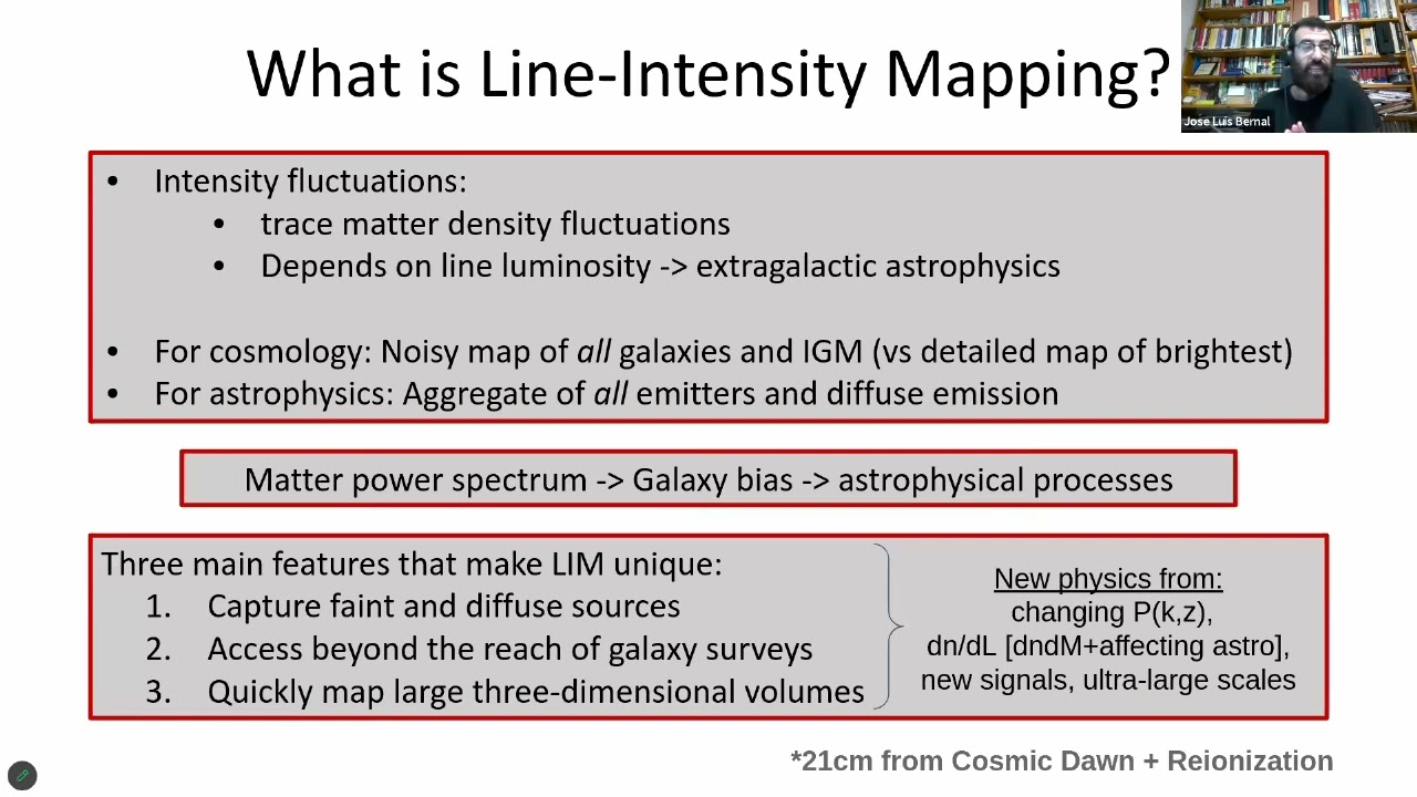




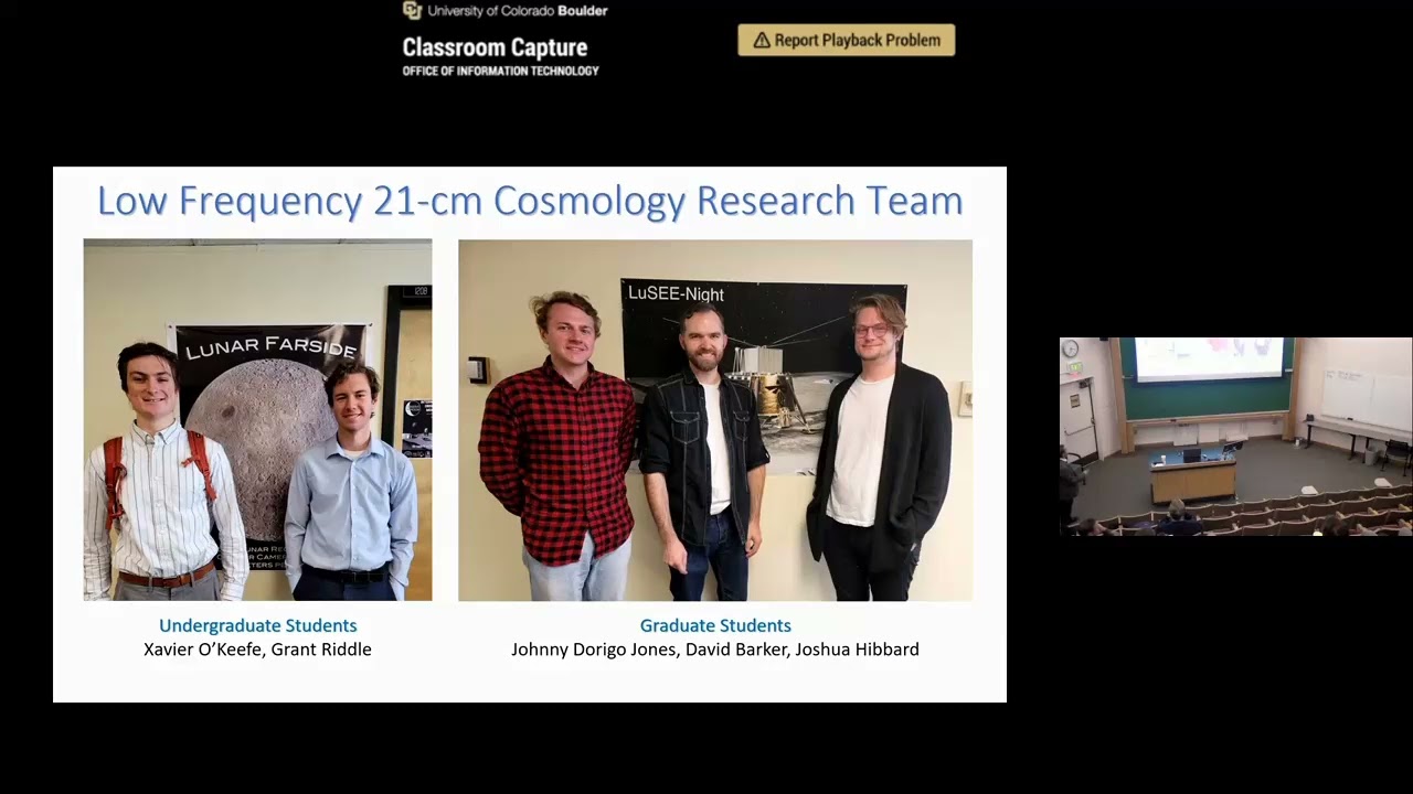



The redshifted 21-cm signal from neutral hydrogen provides a unique window into the cosmic dawn and epoch of reionization, allowing astronomers to probe the formation of the first stars and galaxies when direct optical observations become impossible. This faint signal carries information about the thermal and ionization history of the intergalactic medium, but detecting it is extremely challenging due to foreground contamination from our own galaxy (which is nearly 100,000 times brighter) and instrumental systematics. Experiments like HERA and PRATUSH employ sophisticated calibration techniques and interferometric arrays to separate the cosmological signal from these contaminants, enabling researchers to constrain fundamental astrophysical parameters of the early universe.
Probing Cosmic Dawn with the 21-cm Hydrogen Line
Added:(Speaker 1) Good morning everyone. Welcome to the CMU Bharat CMU Aayana series. It is a pleasure to introduce our speaker today, Dr. Saurabh Singh, Associate Professor in the Astronomy and Astrophysics Group at the Raman Research Institute, Bangalore. Dr. Singh's research focuses on probing some of the least understood epochs of cosmic history, including the Cosmic Dawn, the epoch of reionization, the era of dark energy domination. Using one of the promising tracers, the redshifted 21-centimeter signal from neutral hydrogen. The signal, though (Speaker 1) incredibly faint, carries a wealth of information about the early universe. Detecting it, however, is no small feat. Foregrounds from our own galaxy are nearly 100,000 times brighter, and the challenge is compounded by the need of extreme control over instrumental systematics. To meet these challenges, Dr. Singh leads efforts in designing, building, deploying custom radio telescopes tailored for this delicate measurement.
(Speaker 1) His group is behind cutting edge experiments such as CERES and PRATHUSE and he also collaborates with major international efforts including HERA and CHIME. These projects employ different techniques but share common goal of detecting the red state hydrogen signal across cosmic time. Dr. Singh received his PhD in 2018 from the joint astronomy program at IIS with his doctoral work conducted at RRI. He went on a postdoctoral position at McGill University where he worked on experimental observational radio cosmology. He holds a (Speaker 1) B.Tech in Electronics and Communication Engineering from IIT ISM, Dhanbad. Today, Dr. Singh will be speaking on Whispers of Hydrogen, a 21-centimeter window into the early universe, where he will talk through the science challenges and recent advances in uncovering the cosmic past through one of the nature's most subtle signals. Please join me in warmly welcoming Dr. Saurabh Singh.
(Speaker 5) Dr. Singh, the floor is yours.
(Speaker 1) Thanks a lot, Aritra, for the beautiful introduction. Let me just try sharing my screen. Can you see the full screen presentation?
(Speaker 5) Yes.
(Speaker 4) OK.
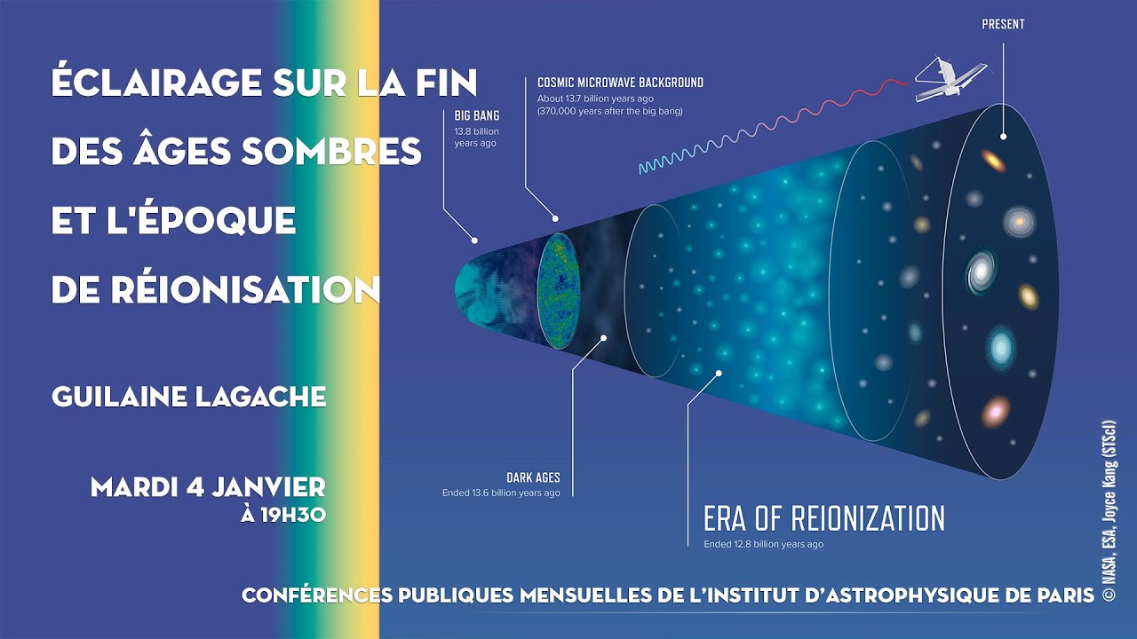
(Speaker 1) So thanks, everyone, for joining today. And yeah, so as Arithra said, I will be talking about how we can use 21 centimeter signal from the neutral hydrogen to probe different times in the cosmic history. And I believe that we have not really covered 21 centimeter physics in this seminar series. So I'll spend (Speaker 1) some time in trying to motivate on why this is important and what is so unique about using 21 centimeter signal to actually do cosmology. So of course I'm sure every presentation in this platform would start from some representation of cosmic timeline and this is no different. So we are here at the center of the universe and I'd mostly be talking about in terms of (Speaker 1) cosmological redshifts. So cosmological redshifts are proxies for time, which is we are probing right from the time when the cosmic microwave background was emitted all the way to the current universe. So higher the redshift, the farther in time we are looking at. So just to give a rough mapping, we expect CMB to be around 400,000 years after the Big Bang and the current age of the universe is around 14 billion years. Now what interests me mostly are these intervening stages. So we know that the (Speaker 1) first atoms had already formed and the photons and the matter had decoupled by the time CMP was emitted which is around redshift of 1100. Soon after what we expect is presence of neutral hydrogen gas mostly and there are photons the CMB photons which are free streaming. But there is nothing really happening it's kind of uneventful period but it has its own unique motivation to study because it's a test bed for many cosmological models. So that is what we would call as dark ages.
(Speaker 3) But then things will become more eventful the time when the first stars and galaxies form.
(Speaker 1) And this is what we would call as cosmic dawn. So cosmic dawn is important because this is the first generation of stars and galaxies and we quite don't fully understand the way they are formed, the time at which they are formed and how different they are in their properties compared to the generation of stars and galaxies that we see in the local universe. Now when these sources of radiation emerged, they did two drastic things to the IgM, the intergalactic medium. The x-rays from these sources heated up the IgM and therefore they changed the thermal history. At the same time, there are also these UV photons which are being emitted and these UV photons essentially start depleting the gas in the intergalactic medium. So soon after their formation, we have epoch of (Speaker 1) reionization. Reionization because universe actually was ionized as a matter of fact it was plasma before CMB, it became neutral and now it is ionizing again. We expect it to have ended around redshift of 6 based on other observations. And of course 21 centimeter signal cosmology doesn't end here you could also use the same signature to probe various later redshift. I'm not sure if I'll be able to get into that, depends on the time, but I would want to mostly talk about the cosmic dawn and reionization as the primary times which we want to probe using 21 centimeter.
(Speaker 1) So this is a crucial epoch. So in terms of times, roughly around 100 million years or so we expect the very first sources of radiation to form. Initially these sources are very local and most of the UV photons actually don't escape. So the ionized regions are all very confined. But that changes as more and more sources form and their ionized regions start to overlap which is what you are seeing here. Now suddenly these UV photons have a huge mean free path to travel (Speaker 1) and they can start depleting the gas at much much larger lengths. By roughly a billion years after the big bang, which is redshift of six, you do expect almost all the gas in the intergalactic medium to have been ionized by the sources for stars and galaxies. So this is basically the full picture that we want to probe here. And the probe that we are using for this is 21 centimeter. By no means this is the only probe, right?
(Speaker 1) So you must have heard outstanding results coming from JWST, for example, which is probing almost this shell, which is redshift of 10 to 15, and it is picking up these individually bright massive star forming galaxies. However the problem there is you can only pick up the (Speaker 1) most massive the most bright galaxies but what we understand from the structure formation is most of the galaxies there are dwarf galaxies they have smaller mass and low brightness, and that is very hard to pick up by the traditional optical telescopes or IR telescopes. And that's exactly what we would want to do. We are not interested in picking up individual galaxies, but we are basically interested in what we call intensity mapping, where you don't look at each source, but look at the overall property of the IGM. So that is precisely what we do with 21cm. The advantage is, unlike optical, which gets very quickly restricted in their sensitivity, (Speaker 1) with 21cm emission you can probe much higher into redshifts or much farther in time. So you could go all the way to almost touching the dark edges using 21cm hydrogen. So this is basically a spin-fl flip transition as you may be aware of. Other beauty of this signal is the redshifting. So depending on at what redshift it's emitted, it gets redshifted by the time it arrives. So a signal which was emitted from redshift of 150 will appear at a different frequency in our observer's (Speaker 1) frame compared to something that was emitted at redshift of 10. And it's a very straightforward relation. It's emitted at a rest frame frequency of 1420 MHz and it's basically divided by this 1 plus e. So the signal that is coming from redshift of 30 would be at 46 MHz. So in some way, the rest frame is 1420.
(Speaker 1) When you design a telescope you can design to have measurements at different frequencies and each frequency that basically corresponds to one slice on this plot. Right. So in some way you can tune this entire range of shells by a single instrument that can make broadband measurements. So in the future slides, I'll be basically using frequencies, but the implicit assumption here is that each frequency studies a particular redshift. Now what is it that we actually measure, right?
(Speaker 1) So I say, okay, it's 21 centimeter brightness, but it actually depends upon a lot of quantities as a matter of fact at different redshift. It measures very different quantities. So let me just spend some time in trying to expand this. So what we measure is Delta TB, which is the brightness temperature of the 21 centimeter signal.
(Speaker 1) The first quantity and probably the most sensitive quantity is the TS minus TR term. So this is the T s minus T r term. So this is the spin temperature of your hydrogen gas, which for all practical purposes, for the kind of redshifts we are talking, is same as the gas temperature. The T r is the background radiation temperature. So in standard models, we would assume the background is basically the CMB. And what we measure is a contrast between the gas temperature at given redshift as seen (Speaker 1) in the background of the CMB. So that is this term. And this is very important because in some way, the change in brightness at different redshifts can be translated on how your gas is getting heated. At much later redshifts, so we are talking now at least redshifts of 10 to six, there is a substantial reduction (Speaker 1) in the neutral hydrogen itself, because by this time, your UV photons have started escaping the halos and getting into the intergalactic medium. And now the H1 starts to decrease, and therefore the intergalactic medium. And now the XH1 starts to decrease and therefore the brightness temperature will reduce. So at lower redshifts comparatively, XH1 takes over, (Speaker 1) while at higher redshifts or the farther times you are measuring this quantity. So in some way, you are probing the thermal history, also the ionization history using a single signal. Now you can study a lot of things in 21 centimeter signal and there are people who actually do all of this. So this is a light cone. This is from a simulation where you start with a very neutral gas, which is very cold.
(Speaker 1) So as you know, this is TS minus TR which is gas temperature minus the CMP temperature. So at those redshift, your gas is colder. Therefore, this term will be negative. So what you see here is blue, which is basically negative. The units are millikelvin.
(Speaker 1) This is just a representation. We measure power in terms of kelvins and millikelvins, but they can be readily converted to the more conventional units. So essentially there is cold gas and therefore the signal is negative.
(Speaker 1) Once the X-rays start to heat the gas, you have slightly higher signals and at some point your gas temperature is hotter than the CMB and this is where you expect the signal to be positive. So these red colors. But by the time that happens, you are also looking at some very nice morphology. And this is because the black regions are basically where you don't have any neutral gas.
(Speaker 1) So it's completely ionized and therefore there is no brightness associated with those pixels. And this morphology is a very strong tracer of what kind of sources ionize the universe. So this is the overall picture that we want. Ideally, in order to understand it, we would actually want this image, right? But that is very tricky.
(Speaker 1) And therefore we want to do some statistical measurements. So the easiest thing that you would want to do is at every redshift, you can take the mean brightness, right? So basically a vertical line and a mean of that vertical line. That is what we have plotted here.
(Speaker 1) So x-axis is frequency, which can be translated to either cosmological redshifts, or it can also be translated to times. Lower frequencies means farther in the cosmic history, higher frequencies, closer to us. Or low redshifts. history, higher frequencies, closer to us, or low rate shifts. So this very particular signature that you see, initially you have a negative signal because the gas is cold, then the signal is getting towards positive because the gas is (Speaker 1) getting heated, and essentially it's dropping to zero because by this time you have substantial reduction in the neutral hydrogen fraction. So this is the mean evolution. This is what I would call as the global signal. Why global? Because there is no particular pointing. In traditional astrophysics, you would want to observe a particular source, particularly galaxy, but this is an all-sky signature. It doesn't need a specific pointing and therefore it's global in nature. But that's not the only thing. It's fairly non-Gaussian field as you can see, (Speaker 1) unlike CMB and isotropies which are very Gaussian. So you can look at higher order moments. The first thing is of course the variance estimates which we would call in Fourier space power spectrum. So there are experiments that measure at different spacings how the power changes. So for global signal, you can actually do that with a perfectly calibrated single element telescope.
(Speaker 1) And I'll come back to what I mean by all of those terms. So this is one example. This is our in-house experiment called CERES that Arithro had pointed out in his introduction. But then for power spectrum, you can't possibly do that with a single telescope. You have to use the full array or interferometer.
(Speaker 1) So one example is this HERA experiment that I'll be talking about a little bit, and then also how we can combine these things together. So the hunt for this started really long ago. The earliest work that I could find is roughly in 1977, on your left here, which was talking about the signature we would expect in the Dark Ages. And of course, back then, we hardly had idea about our constitution of universe about omega (Speaker 1) m or different densities. And therefore for different variations of it, there were signatures expected. This finally came into a much mature field in the 90s and early 2000s. This is the one of the first papers by Schavel and others in 1998, (Speaker 1) that questioned whether can we detect a global signal in the 21 centimeter. And I love this paper by Martin Rees in 1997 that was talking about similar things, but it in its own unique way focuses upon the challenge here, which is, it is not necessarily unfeasible to distinguish the 21 centimeter with everything else. So this basically lays down on why (Speaker 1) this is such a challenging area. But why is it worth it is because the amount of information it withholds about the nature of our stars and galaxies. So on this plot, it's a fairly busy animation by Andrey Misinger, who is a simulator in our field.
(Speaker 1) And all these variables that you see are the free parameters of our problem. These are all related to the properties of the first stars in galaxies. So you have ionization efficiency, you have the minimum mass, (Speaker 1) which can be translated into temperature about the halos that can form stars. You have some properties of the X-ray sources that mean free path. So as they change, and of course, these are completely free parameters because we have no clue what these were for the first stars and galaxies.
(Speaker 1) So for each choice of these parameters, you will see how the light cone evolves. This is a function of time and therefore frequency. And then correspondingly, how the global signal evolves and how the power spectrum evolves. So for some parameters you can see things are very sensitive. For some parameters may not be the case. But this basically gets the message across that if there is a detection of global signal (Speaker 1) or the power spectrum or both, it will in some way we can reverse engineer this and constrain the properties of these first stars and galaxies. So even if we are not measuring the very top group, which is the light cone, we should be able to measure these statistical quantities and do a lot of astrophysics with such measurements. So unlike other cosmological signatures, which is what we are used to seeing (Speaker 1) probably on this platform, the 21 centimeter signal is unique because it's not deterministic. So even if we assume it's Lambda CDM model, just the sheer uncertainty in the astrophysics of these first galaxies give you a range of models.
(Speaker 1) So this is our collaborators at Cambridge now who have done a lot of very nice work on trying to explore all the possibilities of what the signal can look like, both the global signal as well as the power spectrum. So you can see the global signal. This is a function of frequency, correspondingly redshift or time. And this is the brightness temperature. The typical units are milliKelvins or hundreds of milliKelvins. On the right side is the power spectrum, again as a function of different (Speaker 1) redshift. But power spectrum has one more axis, which is different spatial scales. So here we are looking at a very specific spatial scale. And this is the brightness temperature. Of course, it's a variance estimation, so it's millikelvin squared. But what I would like to emphasize here is the sheer brightness, or rather the faintness of the signal when compared to everything else. So why is this so challenging to be able to detect this? And that basically encompasses everything which is there between our telescope and the signal that we are looking for.
(Speaker 1) So on the right side is a measurement that we have done at a radio observatory close by Gauri Bidnur field station. And on the left side is showing all the constituents that are present in this data. So you of course have the signal of interest, but then at the same frequency range, which is roughly 40 megahertz to 200 megahertz, (Speaker 1) corresponding to the red shifts of 35 to six, you have these extragalactic sources as well as their own Milky Way galaxy. And these radiate very strong continuum emission, what we call a synchrotron radiation. There are other also components in the measurement.
(Speaker 1) Then you also have ionosphere, which is highly frequency dependent and time dependent. So it has refraction effects, absorption as well as emission, which of course is higher than the amplitude of the signal that you're looking for. Closer to home, you have radio frequency interference, right? So these are terrestrially generated sources like FM, TV stations, et cetera. And finally, you have your own telescope, which is non-ideal.
(Speaker 1) So what you measure is not just the signal of interest, but every possible thing that we just talked about. And that's what the data represents. So some of these components you can see directly. For example, these vertical lines are nothing but radio frequency interference.
(Speaker 1) And these are probably the easiest to detect because they are very strong. And for example, this is FM. So that is 87.5 to 108 megahertz. You have a bunch of lines at very low frequencies coming from all kinds of sources.
(Speaker 1) You also have a baseline shape here. It's not flat, it's power law like, and that is coming from our own galaxy. And finally, you have somewhere deep in embedded in that the signal of interest. I have a question here, I think in the comments. What's the origin of astrophysical uncertainties? Is it our lack of understanding of the astrophysical phenomena or observational precision or something else?
(Speaker 1) Great question. I would say it's a mix of everything. First of all, we probably don't understand the astrophysics itself at very high redshifts. And because the local universe astrophysics is very strongly constrained from the observations, right? So you have a very in a very high accuracy, you have measured the star formation efficiency, for example, or the distribution of masses in our local universe or even their luminosities in x-ray and radio and other wavelengths. None of these have been observed at very high redshifts. So how do you extrapolate a local universe measurement to high redshift (Speaker 1) when nothing is constrained? That is the biggest question and therefore all the possibilities that you saw was basically you know browsing over all the possible parameter spaces which are completely unconstrained right now. Okay, so moving forward, the first thing that I mentioned was foregrounds. Honestly, it is very high of course, but the spectral features in the foregrounds are very different from the spectral features in the 21 centimeter signal. And this is something that I'll keep coming back to. So on the right, what you see in the blue centimeter signal. And this is something that I'll keep coming back to.
(Speaker 1) So on the right, what you see in the blue line is an expectation of what the galactic foregrounds would look like at different frequencies. This is a sky average. And the typical numbers to keep in mind is something between 10,000 Kelvin to 1000 Kelvin.
(Speaker 1) On the same axis in the log scale, I have plotted the magnitude of the signal, different colors showing the different kind of signals based on the astrophysical model. And these can range anywhere between a few milliKelvins to hundreds of milliKelvins. And you can see the order of magnitude difference. But you should also appreciate that the spectral behavior or the frequency behavior of the (Speaker 1) signal is very different from the frequency behavior of the foregrounds. And therefore, if there was nothing else in the picture, it's just these two things. I think we have some idea on how to deal with the foregrounds. But this problem is completely changed or made more difficult because your instrument itself is very non-ideal. Right.
(Speaker 1) And I'll give you some examples on how. So our design philosophy is, whatever our instrument does, it should not compromise the spectral nature of the signal or the foregrounds. Basically, the foregrounds are intrinsically smooth in frequency space, and we would want to keep it that way. So your instrument should not introduce any feature that can have lots of spectral features in your measured data and that will make your separation between the foregrounds and the signal (Speaker 1) very difficult. But unfortunately, in our experimental setup, there are lots of things that can do precisely that. So I'll just explain two things on this. The first is your field of view itself, what we call is the primary beam of your antenna. So all our radio telescope will have a sensor which is the antenna and its frequency response. So how its field of view changes with frequency can be actually very different. It's very difficult to design an antenna that looks at the same region of the sky across all the frequencies and here we are really talking about a wideband range not a particular narrowband measurement. So why is it so important? Suppose I (Speaker 1) have a galaxy here which is intrinsically a flat spectrum so it has the same intensity across all the frequencies but then my field of view is changing so at higher frequency my response is minimal it is shining on what I would call a second side lobe. But at some intermediate frequency, there is no response. And at some further lower frequency, it has a slightly enhanced response. So this galaxy which was flat intrinsically, what I would measure would look something like this. And (Speaker 1) this is concerning because my signal also has same kind of features as you can see from (Speaker 2) here.
(Speaker 1) Right. So you would not want your instrument to be introducing something like this. Right. And the same thing can happen in multiplicative features of our experiment. So we have what we call as gains, right? So you have amplifier, you have filters, all of them have frequency dependent response.
(Speaker 1) So for example, this is the real data from our experiment. We are measuring the brightness temperature at different frequencies. When you don't have these corrections, the multiplicative impact both from the antenna side, also from receiver, you have something like this. And people in the field will definitely disagree that it looks anything like foregrounds, because there is a frequency response which has been multiplied to it.
(Speaker 1) When you undo that, you get back the blue line, which is closer to what you would expect from galactic emission. So one has to then undo most of these things in order to recover the signal of interest. And this is where most of the challenges lie. So we would call all of these things in order to recover the signal of interest and this is where the most (Speaker 1) of the challenges lie. So we would call this all of these corrections under a single umbrella calibration. So how do you calibrate your telescope to a very high accuracy and here we are talking about accuracy of around one part in a million to one part in hundred thousand. How do you calibrate your telescope to that accuracy over this entire range of frequencies so that you can finally separate these foregrounds from the signal that you are looking for? So I'll now go over the two modes of observations, having kept in mind that these systematics (Speaker 1) are very important. The first set of experiments deal with power spectrum measurements. So just to recap, these are fluctuation measurements of the 21 centimeter line. And there are lots of experiments right now who are trying to detect this, right?
(Speaker 1) So you have LWA in the US, MWA situated in Western Australia, HERA experiment, which is in South Africa, LOFAR in Netherlands, of course, we all know GMRT here, and then upcoming is SKLO, which is roughly 130,000 log-periodic dipole antennas. And one of its science goals is the 21-centimeter detection from the cosmic dawn and epic of (Speaker 1) free ionization. So I would focus on HERA experiment, with which I work closely. And just to give you a flavor of what kind of experiments are required and what kind of challenges they have. Okay and this is exclusively for power spectrum. So the HERA experiment aims to of course detect the power spectrum between 50 megahertz to 200 megahertz. So that would translate to redshifts from 30 all the way to the redshifts of 6. I have a question another (Speaker 1) thing which is wouldn't the foreground be different as we vary the angle but the signal is global and they should have the same features across the entire sky? Great question. That is correct. So if I look at the foreground map, the absolute brightness that you would measure will definitely change with time. Time here means pointing because your telescope usually doesn't move. So as different regions of the sky will come in your field of view, you will measure different brightness temperatures. Having said that, we expect that the spectral behavior of these independent of where you are, will broadly (Speaker 1) be power law like and I put it in double quotes because there will be subtle changes in the spectral nature depending on where you are looking. But the fact that they will continue to remain spectrally smooth, especially when you are looking through a very wide field of view, will be valid independent of where you are looking at. Okay. So as I said, HERA is one of such experiment. It has these antennas, which are expected to be roughly 350 in number when it's completely built. It's in a mode where it's also being built but also observing at the same time which is a very (Speaker 1) quick feedback both for science but also how you can improve your experiment. As I said these are drift scan telescopes which is they have no moving parts. So you're looking at a stripe on the sky. And as the sky moves over your antenna, you sample different regions of the sky. So this is the stripe centered at minus 30 degree declination. This is basically the latitude at which HERA is located. You will see different regions at different times.
(Speaker 1) And these times actually can be covered in 24 hours, but we only take nighttime data. So this can only be covered over several months. You don't have to do your analysis over all the regions of the sky, because some regions of the sky probably are more complicated to model compared to others. So you then now have a liberty of choosing different fields. And therefore you can because as the comment this question was, the signal doesn't change with your angle or your declination or right ascension. So you can comfortably choose your foreground regions (Speaker 1) which are probably low amplitude, but your signal will remain there. So in some way your problem gets a little easy but not by much. But then the question is how do you calibrate such a thing right? Your system here is fairly complicated. It has all kinds of primary beam effects, a lot of multiplicative receiver calibration effects. So I don't have time to get into the details of how do you calibrate interferometers which can be an hour-long talk in itself, but I will give you just two broad examples of how do you do that.
(Speaker 1) The first example basically is the sky-based calibration. So when you are looking at a picture like this, you exactly know what region of the sky you are looking at. Transcribed with Cockatoo
Up Next
Lyman-Alpha Emitting Galaxies From Reionization to Cosmic Noon | Jorryt Matthee (ETH)
@icsuzh1977
275 views•2021-04-30
First Billion Years of the Universe with the Square Kilometre Array
@iaaudc
121 views•2022-05-26

Kepler's Laws of Planetary Motion Explained (Educational Astronomy Video)
@Peekaboo_Kidz
404.9K views•2023-02-17

Gamma-Ray Bursts: Cosmic Snipers Explained | Astronomy
@kurzgesagt
15M views•2016-07-31
Related Study Plans & Knowledge Roadmaps
Structured learning paths in Astronomy