From Lambda CDM to Early Dark Energy: Cosmology Training

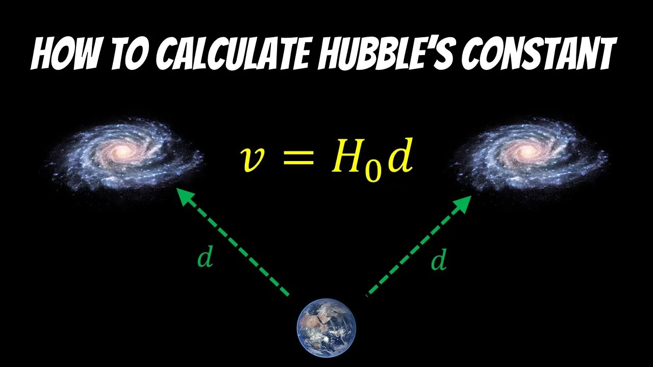
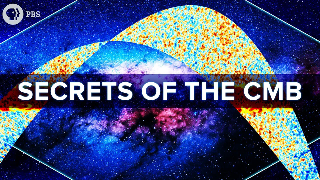
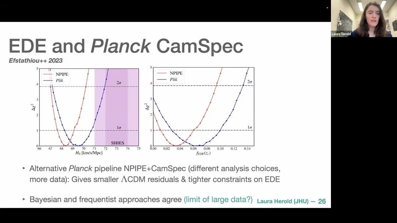
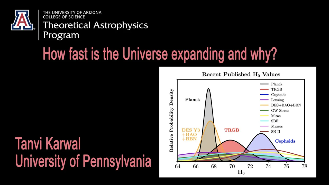
[00:00:08][Music] hi all thank you for being here today for our fourth cosmoverse online training series session with Dr Laura her thank you Laura for accepting our invitation today Cosmo as you may know is a network of over 400 researchers in Europe and over 600 globally with the aim of unifying efforts in confronting the question of cosmological tensions and understanding how different parts of physics can contribute to that effort Dr Herod is currently a postdoctor researcher at Johns Hopkins University in Baltimore in the US she obtained her PhD from the max flank Institute for as physics and Garing Germany under Professor airo Katsu she then went on to take on a post-doctoral position at the same Institute where she worked on various Dark Energy models including early dark energy and where she won the kienan prize for best PhD publication among several other Awards she has been involved in leadership activities such as lecturing and mentoring duties in this fourth session she will present to us the latest approaches toward going from Lambda CDM to early Dark Energy Laura please in your own time thank you thank you so much for the nice introduction and yeah also thank you to the organizers for having me in this uh training series um so yeah welcome to the lecture from Lambda CDM to early Dark Energy uh the plan for today is um to start very basic and repeat some basics of the Lambda game model then go over to the Hubble tension then we can have a 5 minute break and then in the second part of the lecture I will focus more on early dark energy and in the last five minutes also uh I will introduce you to some notebooks that you can do as self-guided homeworks and these will help you to get familiar with Balon solers like class and uh I really recommend to do these notebooks because I think they're actually fun and you don't need to install anything you can do any everything on the cloud so yeah I think you might even learn more from the notebooks than the lectures so um the outline of the first part before the break will be to start with a basic introduction uh where we'll introduce the basic equation in a homogeneous and isotropic universe which are Freedman equations and then discuss a metac content in the universe and how to define distances in an expanding Universe because we will need all of those Concepts to discuss the Hubble tension later and in order to understand the Hubble tension as you know um the discrepancy is most severe between the CMB measurement and the distance ladder it's very important to understand how the CMB actually constraints H not so we will discuss that and then we will discuss solutions to the hyot tension so let's start with a very condensed crash course on cosmology to get everybody on the same page um the basics of the basis of um cosmology is general relativity and I will not go into any details here because there's a long lecture of materal martinell about this topic um but yeah the center pce of gr are the Einstein equations and they basically describe how mattera tells space how to curve and space tells matter how to move so the right hand side has the energy momentum tensor which describes the meta content and the left hand side has the metric which describes the geometry and so after these Einstein equations were written down many people uh were of course interested to find solutions for these equations especially solutions for universe as a whole and to find solutions to these very complicated equations uh they used as a guiding principle the cosmical principle which is very well founded from observations especially the cosmic micro background um so this principle states that on sufficiently large scales the properties of the universe are the same for all observers or equivalently the universe is spatially homogeneous and isotropic on large scale where homogeneous refers to that something is the same in every point and isotropic refers to that something is the same in every direction and so I Illustrated this in this picture here so on the left hand side you could say this picture is homogeneous because it has a cat in every point but it's not isotropic because there's a preferred Direction because all cats walk to the right then on the right hand side of the picture is isotropic from the center but it's not homogeneous because it looks very different in different points um so finding um so fredman Roberts and Walker they wrote down a metric for a spacially homogeneous and isotropic Universe um where the line element that one can use to measure distances in A Spacetime is given by DT Square where T is uh time plus this a of T which is a very important quantity in cosmology it's the scale factor that describes the overall scale of the expanding universe and the convention is to set the scale factor of today to one um then there's another important variable which is K the curvature parameter uh where k equals Zer for a flat universe which is the observationally referred case and flat means if you imagine light rays that start off parallel they will keep being parallel this is different in a spherical Universe where you would have k equals 1 because light rays that started parallel they would converge to each other and they would cross at some point then you can also have K minus one um which is a hyperbolic Universe where light rays that uh start off parallel would diverge from each other then another ingredient that one needs to solve the Einstein equations for a homogeneous and isotropic universe is to Define an energy momentum tensor and the energy momentum tensor that is um compatible with with homogenity and isotropy is is a perfect fluid and this perfect fluid can be completely characterized by its energy density and pressure so um the energy momentum tensor looks like this with robing the energy density and P the pressure and uu is the for velocity of the Observer now inserting this energy momentum tensor and the F lrw SpaceTime metric into the Einstein equation gives the famous fredman equations and need describe uh how the expansion rate so how the scale factor of the universe uh depends on the curvature the energy density and the cosmological constant and there's a third famous equation that one gets by inserting the the second fredman equation into the time derivative of the first fredman equation which gives the continuity equation and this uh describes how the energy density of the universe changes with the expansion now um this row here in the fredman equation is the total energy density of the universe but it's very common to Define row K so interpret the curvature also as the energy density and row Lambda so energy density of the cosmo constant so one can rewrite the first freed equation in a more condensed form so the um uh scale or the expansion rate just depends on the total energy density of the Universe um so in the Lambda CDM model uh this total energy density is composed of different components of radiation meas the cosm cosmologic constant and curve but from observations mainly from the cosmic microwave background we know that curvature must be very small um so we will NE neglect it from now on um now in an homogeneous an isotropic Universe um the components can be completely described by a linear equation of state where the pressure of the component is proportional to the energy density and the different components they have different equations of State parameter W so dark matter and bionic matter they are pressureless so w is zero no photons radiation and neutrinos uh they have pressure so w is 1/3 that also lets them red shift faster than matter and then there's dark energy or the cosmic constant that has W = minus one so in a sense negative pressure that leads to the expansion of the universe and inserting this equation of State in the continuity equation lets it lets us rewrite it in a more convenient form and using this equation one can directly describe the energy density of the Universe um as a function of the scale factor and we will need that later and the convention here is to have a subscript zero in order to refer to the current time today um so as we said the first freedon equation describes the rate of expansion as a function of the energy quent of the universe and this is nothing else but the Hubble parameter so the Hubble parameter is a DOT over a and the hover constant then is a hover parameter today so the hover parameter at T equals t0 and this a parameter that we will talk about a lot later in the context of the Hubble tension so inserting uh a The Hub parameter in this equation um um we can define a critical energy density which is the density of a flat universe of universe without curvature if we have k equal Z it's simply the uh total energy density of the universe and inserting this in this equation uh one can bring the H KN on the other side and then we can write this Freedman equation in a very condensed form moreover it's uh it's useful to Define these fractional energy densities the omegas where Omega I I is some component like radiation or matter is given as the energy density divided by this critical energy density and using that one can even condense the equation further and using the time evolutions of the different components like radiation matter and curvature one can write this uh as a function of the scale factors and introducing the red shift which is 1+ C equals uh the scale factor today over a we can finally rewrite this in the very famous form that we will use a lot later where H S over H KN squar is given by the different components uh with their Rift dependence so from this we can directly read off that radiation um deludes with one plus the red shift where matter deludes with one like to the power four and matter with 1 plus to the power three so radiation dutes faster than meta dutes faster than curvature and Omega Lambda is constant it's a cosmologic constant um and here we always wrote when we always wrote a subscript of zero when we referred to the current time but it's often just omitted so that I actually denotes the current um energy density of the Universe um so people simply write the explicit time dependence if they wanted to refer to them to the time dependent quantities and now I want to switch gears a bit so in an expanding Universe it's actually not straightforward to Define distances um there's two very natural ways to Define coordinate systems and measure distances the first is a a CO moving system that expands with the universe so if you imagine that you have two galaxies um they start off with some coordinates and they keep the same coordinates even though the universe is expanding and um their distances are growing then a second coordinate system that's very useful is just to have a fixed coordinate system where the universe expands within that coordinate systems and objects actually drift apart with the expansion and now we want to relate a physical distance so an actual measurable physical distance with the scale factor a and now to get an expression for the Coe moving distance SK one can can consider a photon um traveling at an infini dismal distance RP where we know that a photon travels at the speed of light so um since we work in natural units here the speed of is one so we can compute that by Dr by DT and now if we insert uh the the expression for R here we have a d by DT and now basically doing separation of variables we can integrate over T to get an expression for S of T now inserting again the red shift um we can write this in we will use a lot later that the comoving is given by an integral over red shift divided by the Hubble parameter right now we talked about Co moving distances and physical distances um but it's very convenient to to define the soal angular diameter distance which one can directly infer from observations and the angular diameter distance is defined such that this very natural equation holdes such that um an angle um can be computed by dividing the size of an object by the distance of the object so this basically the small angle approximation that we require uh to hold also in a cosmological constant even in in expanding universe and uh the expression for the angular diameter distance is simply the scale factor times the co moving distance and to derive this equation for da one can um consider that the proper size of the object is actually given by the co moving size times the angle which would be um the co moving size of the object and then one simply can multiply the co moving size of the object by the scale factor a and this goes one um if one inserts this in this equation here one has uh one brings the a of t on the out side and gets this equation so um how to solve the Hy tension now um first of all let's introduce the Hub tension so the Hub tension is a discrepancy between different measurements of the current expansion rate H KN and it's most severe between the cosmic micro background measurement um which is an indirect measurement of H KN because it the CMB constraints the composition of the universe at Early times and needs to assume a cosmog model uh in order to in refer the expansion rate today and since the CMB constrains the composition of the universe so well this is a very precise measure of the expansion rate but it is model independent because one needs to assume a model to predict the expansion rate today there's also other indirect measurements um like using Baran acoustic oscillations that we will discuss later and using Galaxy clustering then on the other hand side the are the direct measurements of H KN which are based on the on distance ladder for example seths trgb that are used to calibrate supern noi one can also use strong gravitational lensing and these approaches are typically less precise U due to the astrophysical modeling but they are independent of the cosmological model so it's really two different um types of probes that are in ttention here so how can we from a theorist perspective solve The Hub tension this General strategy to solve the tension is that the is to assume that the direct measurements are correct um and to change the cosmological model in order to infer a higher AG not so basically our goal here is to um change the model such that from CMB we get an H not of 73 kilm per second per Mega um but in order to get a higher H not from CMB we need to understand how the CMB does actually constrain H KN so the CMB provides the most important cosmologic appro when it comes to constraining the parameters of the cosm model so to bring everybody on the same page here's an illustration from the W map collaboration of the history of the universe so in the early Universe um the universe was very hot and dense and the idea is that Quantum fluctuation during inflation actually led to density um to density perturbations uh that expanded with the expanding Universe once inflation ended the UN Universe uh expanded at a slower pace and cooled down and once the universe cooled down enough such that um electrons and protons could form atoms light was suddenly free to travel and um this is what we see today as an Afterglow of this very hard universe as the cosmic micro background and after the CNB the universe expanded at a slower pace and galaxies and stars formed and then at late times something else interesting is happening that the uh Dark Energy leads to an accelerated expansion um so this is what the sky looks in Optical if one is in a very dark place and on the southern hemisphere spere such that one can see the galactic center and this is what it would look like if we had eyes in microwave and I actually literally downloaded the 70 GHz plunk map without any uh processing and this is what it looks like so one can clearly see the galactic plane in microwave so if we professionally mask the galactic plane with this white box we see that the micro sky is basically a constant temperature of a 2.7 kin now if we crank up the contrast we can uh literally see the CMB and this is um the image from the plant collboration with some proper foreground cleaning and in painting and here you can see that while the CMB is almost constant at 2.7 Kelvin there tiny fluctuations at the level of micro cabin um so how can one analyze CNB Maps like that um the very the most common strategy is to decompose the temperature fluctuations into a set of waves with various wavelengths and then the second step is to plot the strength of each wave length which gives the power spectrum and in one dimension we're very familiar with that because decomposing into waves in one dimension is a f transform but on the unit sphere decomposing into waves corresponds to the spher harmonics decomposition so what we do is we start with the map on the left and side um where the map can be described as temperature fluctuation as a function of the angles Theta and F and these temperature fluctuations they can be expanded in terms of these spherical harmonics functions and coefficients Alm and the Alm contain exactly the same information as the map so the spherical harmonics function are fixed function that one can look up on Wikipedia basically and the alms they contain the information from the map now L defines the multiple and the higher the L the smaller the scale and now the power spectrum is given by um basically averaging over the M values and taking the absolute value square of these alms because alms are complex functions and this gives a real function the power Spectrum or just also called the CSS and uh this is what they look like from the plant collboration it's very common to write to plot instead of the c l plot the DL which is simply L * L + one because this um gives shows better um the scale of variant part of the P Spectrum now that we have these red data points how can we analyze data like that and get cosmology out of from out from this data so to predict the CMB power Spectrum one needs to solve the full fluid equations which are the bolman equations for all components of the universe and this can be done with cosmological bolman servers like camp and class which um you will hear more about in the in Notebook homeworks and these Bon solers they take as input the Lambda CDM parameters and be they can be sampled within uh mcmc Samplers so the Lambda CDM model uh has six or the basis Lambda CDM model has six parameters and Omega little Omega CDM is typically defined as H2 Omega CDM which is a physical energy density in cold Dark Matter then Omega barion is little h Square Times uh the fractional energy density in barrance which is the physical energy density in barrance now this little H is the dimensional H constant which is simply H not divided by 100 km/s per megapath um then there is toio which is the optical depth to rization which is basically a measure for how often the cnbs photons scatter um from the emission to us and then there's as and NS which is the amplitude and tilt of the primordial power Spectrum s predicted from inflation and yeah if you do the exercises later you might find this useful um so we already saw the CMB power Spectrum but of course the most distinct feature are these Wiggles here so what generated The Wiggles um the wigg are the soal baron acoustic oscillations and they are generated in the very early Universe when the universe was a hard plasma of Barons and photons and the belief is that small density fluctuations are generated by Quantum fluctuations during inflation and in places where there's a little bit more um more matter gravity attracts even more matter so overd region get more and more overd however since the photons and the Barons are tight coupled the photons have pressure so once these over density get too dense the photon pressure will drive them apart and if you have a driving force and a restoring Force you will find some oscillations and you can imagine this like raindrops on a water surface so the one fluctuations are basically the raindrops and they lead to some initial perturbations on the water surface and now as on the water surface you have a driving force and the rest storing force and you will get waves and since there are many quum fluctuations these waves overlap all in space so we cannot see distinct waves but we see an overlapping pattern of many waves in the CB and once the electrons of photons recombine the photons can travel freely and this is when the density waves freeze and we can basically see a Frozen picture of these density waves in the CMB so now that we know that these Baron acoustic oscillations these Wiggles are from traveling um sound waves basically we can compute the co- moving distance that these sound waves in the early Universe traveled and this is the so-called sound Horizon um so the we know that the sound waves they started traveling at the Big Bang until the time of recombination which is denoted as tar uh and tar or recom is the time when protons and electrons combine and the photons can travel freely and this is when the CNB is sent out so we can simply obtain RS by taking time times velocity like we would do normally but since the Sound Speed uh depends on time we need to integrate over over the Sound Speed however there's one small complication while the sound waves travel in the early Universe the universe expands and this slows down the sound waves in the coob coordinate frame and um this is expressed by um basically this ratio of the Sound Speed divided by the scale factor of the universe so this factor in the expansion of the universe while the sound wave waves travel um so we have the comoving sound Horizon and now we want to rewrite this Co moving sound Horizon um we can use the fact that we know that d a is simply a DOT so we rewrite this integral as a function of the scale factor um then we want to rewrite it is in terms of the red shift so we know that the red shift uh derived by the scale factor is simply one / a derived by a which gives this minus 1 / a s and we can insert this in this integral and simplifying this we can identify the Hubble parameter here we get um the most common expression for the comoving sound Horizon uh where we can compute the comoving sound Horizon by integrating the red shift from the red shift of recombination uh to the Big Bang um over the Sound Speed divided by the H parameter and now one uh Missing Piece here is the Sound Speed so from experiments on Earth we know that the sound speed in a plasma is about 1/ < TK 3 uh the speed of light but here there's a small cor correction coming from R which is the bar and Photon ratio and it's given by this expression here so now we have basically all the pieces together to compute the comoving sound Horizon um and the thing is what we actually observe is not the physical sound Horizon the physical size of the S rizon which is depicted as this ring here but we measure the angular size of the Sison so we measure this angle Theta because um the CMB we see as a sphere on the sky so all we do is measuring angles basically but we can relate the angular size of the Sound Speed by dividing the physical size of oh sorry the angular size of the Horizon is given by the physical size of the sound Horizon divided by the angular diameter distance and the angular diameter distance we already discussed before uh is given as this integral from today to the red shift in consideration integrating over one over h of that and here we're sometimes switching between the physical size of the sound Horizon and the co moving sound size of the sound Horizon but from by or one can simply convert between physical coordinates and Co moving coordinates by using the scale factor so ultimately we wanted to talk about the Hub tension so how does the CMB constrain H not so it constrains hot uh over the angular size of the S Horizon so basically over the distance between those Wiggles in the CMV PA spectrum and as we said this is given as a ratio of the physical size of the soundis divided by the angular of diameter distance and these are expressed as these two integrals where both of them them depend on H of set so um cosmology mainly enters over h of set here and as we derived earlier h of Z can be written as H time the square root of the components of the universe and the respective dependence on red shift so now if we can get Omega radiation Omega meta and Omega L Lambda from somewhere else um this equation becomes an implicit equation for H KN so now the question how does the CMB constrain H KN reduces to how does the CMB constrain Omega radiation Omega matter and Omega Lambda and um so Omega radiation is a actually very easy to get because Omega radiation uh is related to the temperature temp of the CMB by the T to the 4 law and the temperature of the CMB has been measured very precisely by the uh firus experiment on the Kobe satellite so by simply plugging in the temperature of the CMB we can already uh determining Omega radiation and this is also why Omega radiation is basically fixed in all analysis because it has been measured so precisely already then how can we get Oma so actually the CNB is not sensitive to Capital Omega matter but so little Omega matter um so the physical um energy density in matter and this quantity can be obtained from the height of the acoustic Peaks so Theta s is basically the the distance between the acoustic Peaks but one can get Omega M matter as the height of the acoustic Peaks so here in this plot I show that if you have higher Omega matter you get lower um peaks of the CMB and this is the the so-called sux wolf effect so yeah from that we can get Omega matter independently of H and then how can one get Omega Lambda now since we assume that the universe is flat and k equals zero in a flat universe all these energy densities are related by uh this Clos equation that Omega radiation plus Omega meta plus Omega L is one so by having omeg radiation Omega matter one can simply obtain Omega lter so now um basic we have all ingredients um that are needed to get to directly infer H KN from Theta s so now um how can we use that information to resolve the hypotension by modifying the Lambda C M model so as we said before what we actually measure with the CMB is Theta s so the distance between the acoustic Peaks which is given as the fraction of the Ang the physical size of the sun Horizon divided by the angular Dam at a distance now as we said Theta s is precisely measured by CMV so Theta s is assumed to be fixed so there are two options to solve the Hy tension one are the so-called early time Solutions and these Solutions they modify the universe between the red shift of recombination and the Big Bang um and then on the other hand side we can modify uh the denominator these are the so-called late time Solutions and they they somehow affect h of set between um today and the red shift of recombination now let's have a look at the late time Solutions first um so they modify da between um today and the red shift of recombination by modifying the expansion rate in this red shift range so by modifying h of Z now we can have a look at h of Z at late times at late times radiation is um pretty much negligible because um we are in matter domination and therefore h of set can be expressed simply as um as a function of the omegas and H not and now the problem is that we have lots of observations of a of set and Omega matter of set coming from Galaxy Baron acoustic oscillation data and Supernova data so it's very challenging to increase each not enough so you can you can have some small impact here but it's it's challenging and there's a lot of constraints to get that working but there are some approaches and I think they they discussed in other lectures so I'll um leave the late time solutions to them um then there's the early time Solutions which modify RS so if we look at the formula for RS there are three options uh to do that one can modify the red shift of recombination Z star one can modify the Sound Speed uh C Zs or one can modify age of set and all all of the three things have been tried but the easiest by far is to modify y h of set for example by introducing an energy density which boosts the expansion rate before recombination um now if we have a look at age of set at Early times we can set the cosmodic constant to zero because uh Cosmic constant only starts to become important at very late times so h of set is given by this formula and the idea here is to introduce some additional energy density so introduce an additional Omega which increases age of said at Early times and now if we increase age of said at Early times this leads to smaller physical size of the soundon RS so this whole quantity becomes smaller and one of the um arguably maybe most successful ideas is the early du energy model so what's the idea behind early duck energy so as we said Theta s is six per observation it's given by the distance of acoustic Peaks and it's measured with.03 Precision by plankk so what a du energy does is it introduces an additional component before recombination that reduces RS so we said h of set is increased by early duck energy at Early times so this um h of set increases that means this whole term becomes smaller so RS becomes smaller now because Theta s is fixed by observation if RS becomes smaller and Theta is fixed also the angular diameter distance has to become smaller so because th s is fixed the angular diamet distance decreases um and if we look at the formula for the angular diameter distance it mainly depends on age of set and if we assume that in the early duck energy model the energy content is similar to Lambda CDN the easiest to easiest way to get a smaller da is by increasing H knot and therefore H not decreases in early dark eni models and this is what we were aiming for in resolving the H tension okay so this already brings me to the recap of the first part of the lecture so in the first part of the lecture um we had this very condensed uh overview of the freedent equations Hub parameter and how to define distances in an expanding Universe we went through some CMB Basics and we talked about Baron acoustic oscillations and then we talked about how the CMB constraints H not and how early and late Universe Solutions work by either modifying RS or da and then in the second part we will talk about more how to realize the early duck enery model are there some questions you you spoke in your calculations about that the universe is fr does this follow from the measurement in in in your derivations or is it such an assumption that it is approximately yeah it actually follows from the measurements yeah actually earlier said uh curvature is constrained by the CMB but actually it's not entirely true you need to have the CMB and Baran acoustic oscillations in the Galaxy data so as you as you probably know the same um sound Horizon that's imprinted in the CMB is also imprinted in the Galaxy uh distribution so we actually have a handle on measuring this ring here at different red shift um so because what what curvature does basically if you imagine this these here are light rays in a flat universe they simply travel in straight lines but now you have let's say you have a um positively curved Universe then the light rays would travel more like this would change your uh some of the observations so you can you would have to put this in because if you then say you you change your model or don't change it uh it it could have some impact on on this flatness pie that this is what I always wondered about when we read all this papers so it's it's a question it's actually it's very well constrained by observation so the CMV alone is not very sensitive to the curvature because it's only measuring the Bao ring at one red shift but if you can measure the Bao ring at different red shift you basically can constrain how the light rays travel so we we know that the light rays don't travel in this curved path because we have information about how big is this ring at different red shifts Brar and acoustic oscillations thank you really very much for this lecture for preparing it I have a second question maybe I I didn't get everything uh widely but you mentioned at some point that uh one could derive the C be by solving portzman equations and how does this uh is this connected to what you said later about uh contact with measurement and and and and with your formul you derived for what this Angel and for the uh for the um speed of sound and all this is this or what does this come in I just didn't see it or maybe didn't get it or whatever yeah you're right I'm I was uh skipping definitely the connection there so of course when people do CNB analysis they do not do this analytic computation um because this is what people did in the early days of CMB they basically just looked at uh what is the distance between these Peaks and they then they compared the prediction of theta s to the distance of the peak but of course this is just one number and nowadays people do full shape CB analysis so they do uh full forward modeling basically of of forward modeling is maybe not the right word but you you assume some meta content and then uh you solve the full fluid equations and you predict the whole shape of the CNB power spectrum and not just Theta s so I just went through this derivation of the D because I think it's uh instructive from like pedagogical way way of uh looking at it but this is not done anymore but I believe this was done in the early days of the CMB when the data was not very good um and this is basically what people do now in in Galaxy clustering they only infer the Bao scale so they only infer one number from the observation and they compare it to the prediction from Theory but yeah um in the CMB analysis what people do is predict the full shape and not just CS I just saw this a question in the chat about how uh Theta s is being used in measuring H because H KN appears uh the same way in the numerator and denominator uh so it should cancel out um I mean in principle yeah it appears in both numer and denom Native but you have this integral over different ret ranges so basically here you have uh the expansion rate from today to the red shift of recombination here from the red shift of recombination uh to the big band The Sound Speed doesn't have a strong dependence on age of that so the Sound Speed is mainly dependent on the bar Photon ratio also uh you are asking about why H not doesn't cancel out but um these quantities are measured very differently and so the the yeah the main part is that they are in different ret ranges okay then let's um have a closer look at early dark energy so early dug energy is U most often modeled as a Scala field so I want to have a small section about Scala fields in general in an expanding SpaceTime and just to get a small int intuition about what a Scala field is uh I have one slide about that it's actually a very simple thing it's just the scal field assigns a number to every point in time and space um these are very common scal fields are very common so for example temperature is a scal of field or density or pressure because it assigns a number to every point in space time or potential Fields like the gravitational potential and electric potential are also uh scale fields and the inflaton driving inflation is also most commonly model as a scal field so it's very common uh things in physics and the action of a Scala field minimal coupled to the metric uh can be written as follows so it we'll also just um talk about this very briefly because William has given a lecture about inflation and this is exactly the same physics or almost exactly the same physics as inflation so the action can be written as this integral over the whole space time uh with the determin determinant of the metric here and the kinetic term that's proportional to the derivatives of the scalar field and a potential term and from that action one can compute the energy momentum t of the scal field via this um formula that comes from gr um and if we insert uh isotropy and homogenity into this energy momentum tensor for the scalar field we end up with this formula and this is interesting because by comparing this energy momentum tensor of the perfect fluid oh sorry this energy momentum tensor of the scal field with the energy momentum tensor of the perfect fluid one can simply read off the energy density and pressure of the Scala field so here we see that the part proportional to the metric is the pressure so this here gives the pressure the F dot half minus V of F and then one can also from having the pressure one can read off the energy density now inserting the energy density and the pressure into the the first fredman equation and the continuity equation one gets the uh Evolution equations for the Scala field where here in the second equation uh one has the second term is the Hubble the So-Cal Hubble friction because it's proportional to F Dot and slows down um the movement of the scaler field in the potential and then there's a potential term here and the second equation is nothing else but the Cent K Gordon equation for a Scala field in an expanding space time so basically the frin equation reduces to the Klein Gordon equation if one inserts um homogenity in isotropy isotropy and the uh Scala field um so early duck energy is model usually model as a scal of field and here is a short history about early duck energy early dug enery models have already been studied before the Hubble tension emerged but more in the context of quintessence models so models of late time Dark Energy then the accent like early Dark Energy was proposed as a solution to the H tension already in 2016 um but it was could only be shown in 2018 and 20199 with a proper modeling of the perturbations that it's actually possible to solve the hension with this model and there are many versions of the early Dark Energy model but here we focus on the most commonly studied early duck enery model which is the ax like early duck enery model um yeah early dark energy is simply a Scala field in a potential we of five which boosts the expansion rate before a combination and the potential was originally motivated from the Axion um but here we take it as a phenomological potential um because for the qcd Axion you have some very strict relationship between F and this normalization here and this is not possible to solve the hyper tension with this type of oxion so here we simply borrow uh the potential from the Axion but early du energy has not much to do with the axen anymore so um this potential depends on this normalization Factor V that is given by m^2 f s where m m is called the mass and F the Decay constant of the field and Decay constant also appears here and then there's the index n of the potential for the standard axan one would expect n equals one however in a cosmologic context this doesn't Decay quickly enough and Nal 3 is preferred is a preferred value by the data because it decays quickly enough and therefore doesn't affect late time physics too much and therefore it fits the data better and in analysis in data analysis one commonly fixes this uh index to three um and only samples the other three parameters so the three parameters of this model are the mass the soal Decay constant and the initial value of this Scala field in its potential and there one commonly defines Theta I as f i so the initial value of the scalar field divided by F and N is fixed and so let's have a look at the Dynamics of the field so the Dynamics are governed by the CL Gordon equation initially um uh the expansion rate of the universe is very high so this term the hper friction term dominates and this field f is basically Frozen in its initial position and in this phase it behaves like dark energy so this is very similar to the inflaton which is also Frozen in the potential and therefore leads to um this rapid growth of the field then at some point the Hubble the Hubble expansion slows slow go down and the potential term gets of the same size as the Hub friction term and this is when the field gets released and it starts rolling down as potential and starts to oscillate around the minimum and one can show that in this phase the field decays or red shifts away faster than matter so the equation of state of this um field is wal minus one for red shifts uh earlier than this critical red shift so the critical red shift is a red shift at which these two two terms have the same size and this is when the um fi Stars oscillating so before the critical red shift uh the equation of state is minus one like dark energy and after the critical red shift um the equation of State changes but the time average of the equation of state where n equal three is 1 12 so it Rifts actually faster away than a radiation which would have W of 1/3 um so you can see here on the right hand side the fraction of early duck energy as a function of red shift so on the right hand side are large red shifts so early times and at Early times this field grows very rapidly um like a dark energy component then the field starts oscillating in the potential and starts to R shift away and what one typically does for the data analysis is one trads the particle physics parameters MF and Theta I uh for the phenomenological parameters fed which denotes the maximum fraction of early duck energy at the critical red shift uh CC and additionally the initial value of this scale of f so in data analysis typically people vary these parameters instead of I'm sorry I have a question can I ask yes m is the mass of what like actually I joined in like in the middle of your presentation so I didn't understand like m is the mass of what yeah m is basically a parameter appearing in this potential um the thing is m is just an effective Mass so you can basically the mass of a Scala field if I remember correctly it's given by the second derivative of the potential by the Scala field and only for n equals 1 m is actually the effective mass of this field if you have higher n it's uh there are some correction factors but yeah M can be interpreted as the mass of the scal field for Nal one okay thank you to solve The Hub tension one typically aims at about 10% of the fraction of early du energy at its maximum um so let's have a look what these different parameters do so the critical red shift which is red shift at which the field starts oscillating in the potential it determines when um when the field Peaks so changing the critical red shift just changes the time at which early duck energy Peaks and then fed of course which is Omega Ed at the critical red shift determines the height of this peak now Theta is a little smaller effect so the initial value Theta I since it's an angle it is between Z and Pi uh determines how fast the field oscillate when it decays so if you look at the pink line which is Theta almost at Pi one has many more oscillations than if Theta I has a small value so if the field starts very close to the minimum this would be this black this blue dashed line the field doesn't oscillate very often and decays um without oscillating much um so the closer thet I is to Pi the faster the oscillations and then the index of the potential determines how fast the field decays the higher the index of the potential the faster the Decay um so here if you have a look at n equals 2 which is a blue dash line the field decays only very slowly and this is um very much disfavored by data sets so n is typically fixed to three which is this uh green line here so can early du energy resolve the Hubble tension and fit all data sets at the same time and I put together a very short review about constraints on early D eni which is definitely not uh complete um so of course this question depends on the data sets that are considered so I want to discuss some very commonly considered data sets here uh of course the plank CMB measurement the temperature temperature the temperature eote and eote eote uh Power Spectra and the L in contribution um then we also want to consider Baran acoustic oscillations imprinted in the Galaxy positions so before we talked about the Baran acoustic oscillations imprinted in the CMB but these Baran acoustic oscillations because they are imprinted in The Meta distribution of the universe in places where there's more density there's a higher probability that galaxies form so this Baron acoustic oscillations are also imprinted in the galaxy distribution and we can measure them today and then there's also ret space distortions that are also often used in data analysis uh which are basically an apparent Distortion of this Bao ring because of the peculiar velocities of these galaxies and this is actually a good measure of the the growth of structure and then um there is the famous Pantheon and shoes data set which is one of which is the most competitive direct measurement of the Hub constant and it uses seed calibrated type 1 a supern noi so what they do is they use paralus typically from the Gaia experiment to measure very precise geometric distances to SEI which are pulsating stars in our own Milky Way and with that they can calibrate the distance Luminosity relation so they know um basically how distance how distant um an object is depending on the luminosity and they use these seeds um in order to calibrate supern noi so they look for Galaxies that have both seeds and supern noi in them in order to use their information on the seeds to calibrate the absolute Luminosity of the superi and the supern are very bright so we can see them very far away uh far out in the Hubble flow so they can be used to constrain directly the Hubble law and the Hubble law as you probably all know states that the velocity the recession velocity of an object is proportional to the distance of that object and the proportionality constant is the Hubble constant so now if we know uh the recession velocity which is very easy to get because we can simply uh use red shifted spectral lines in order to get the recession velocity and the distance we get from the distance uh Luminosity Duality so once these supern are calibrated one can directly uh compute the distance so then uh the inclination of the slope gives you the hle constant and using these data sets one can analyze the early duck energy model and one finds that these data sets prefer a fraction of about of about 11% of early duck energy and an H not of about 71.5 so here on the right hand side you can see the uh 1D marginal as posterior and I don't have time much time to go into Data analysis here because I think there's a uh lecture by Jurgen about this this whole topic of data analysis but in this one de marginalized posterior uh you can see that orange is a Lambda CDM posterior what Ed does is it increases the arrow bar on H knot and shifts uh H knot to larger values such that the tension with the Sho direct measure which is the gray line here is reduced to below one or two Sigma so if a model achieves a reduction of the tension below to Sigma people already uh speak about solving the tension because it's it's very difficult basically almost impossible to find a model that shifts your central value of H KN to these high values um however if you introduce early duck energy um not only H KN increases but also other parameters shift for example early dug energy suppresses the growth of perturbations at Early times this is because early dug energy basically uh boosts the expansion of early times so um perturbations have less uh time to grow and this leads in order to compensate the suppressed growth one needs more Cold Duck matter and a higher spectral index and this is the so- called early integrated sex wealth effect um and this worsens the sigma 8 tension and here a small aside on the sigma 8 tension so Sigma 8 is a parameter that measures the amplitude of density fluctuations in the late universe and it can can be computed by an integral over the linear metap Spectrum convolved with this um um top head filter with a radius of 8 megap over H so Sigma basically smoothes uh the density field with a radius of 8 megap and looks at the amplitude of the fluctuations at this uh length scale now S8 is simply a convenient combination of Sigma 8 and Omega M that's better constrained by weak lensing experiment in turns out that plunk prefers about two to three sigma higher Ade than weak lensing experiments like the dark enery survey the kilree survey or HST and weak lensing um uses the Distortion of Galaxy shapes because of gravitational lensing so some foreground Source lenses the background sources and that gives one a measure of um the Met distribution in the foreground and this is a very good data set to constraint s so motivated by this increase in Omega CDM and this this worsening of the S8 tension basically um many authors started to include uh large G structure lar structure probes into the analysis so if one includes DS kits and HSC to this analysis one finds very tight upper upper limits on the fraction of early duck energy and values of H KN that are perfectly consistent with the CMB but they cannot reach the H knots of shoes they're not able to resolve The Hub tension however a more General picture evolves so it turns out that actually uh if you do not include shoes into the analysis um you find no preference for early duck energy at all and if you additionally include large G structure probes you get very tight up the limits on the fraction of early du energy so here on the right hand side if you look at the red line uh you get just from CMB data alone you get a quite tight upper limit on the fraction of early duck energy if you also include all the large case structure probes your limit gets even Tighter and only including shoes into the analysis um gives you a preference for early duck energy however uh many authors have pointed out that volume effects could affect these uh results and volume effects they are technical effects in the basion analysis and to explain volume effects are also known as priv volume effects or projection effects I picked this uh Toy example here in this toy example assume you have an experiment that measures two parameters Alpha and beta and this experiment gives you this black posterior here now let's say you're more interested in Alpha so you might want to look at the 1D marginalized posterior and Alpha which is obtained by simply integrating over beta so one integrates out this beta Direction and obtains a one Dem posterior in Alpha and uh the peak of this 1D posterior is in zero here and this non-asian extension only leads to small a symmetry of this um marginalized posterior but now assume that you have a second experiment this experiment two which is only sensitive to Alpha so it has this blue posterior here you look at the marginalized posterior you might conclude that Experiment 2 and experiment one are in maybe two or three sigma tension but if you look at the 2D posterior there's actually no tension and you can safely combine experiment one and experiment two to get this uh very tight Contour so it might seem counter intuitive that actually although Alpha equal zero and Alpha equal 5 fit the data equally well Alpha equals 5 is outside of the two Sigma confidence interval of the marginalized posterior but this is simply a projection effect just because there's much more volume in um Alpha with zero equals z is preferred um from a volume perspective and here in this example it's very intuitive to understand because we can directly look at the full posterior but in cosmology analysis it's often very complicated we because we have this large dimensional models with many parameters so we cannot look at the full end dimensional parameter space um so these prolume or projection effects they appear if the posterior is influenced by the prior volume and reasons for that is that the data is not constraining enough um for all these parameters and this leads to a very flat likelihood surface and that means that the the posterior actually has a strong influence from the prime this can happen in models with many parameters also the parameter structure of the model can generate large volume differences and this often happens with nested model and early D she is such a nested model because if you the fraction of early duck energy go to zero uh you recover the Lambda CDM limit so the early duck energy model is nested within the Lambda CDM models that means um if you go if FD goes to zero your two other parameters that describe the early du enery more closely Theta I and CC they become completely unconstrained and that's why there's much more volume in F of Z then at larger values of fed and this can lead to a preference of fed of Z in the marginalized posterior and one idea to probe the influence of these prior effects is to use the profile likelihood so what is the profile likelihood it's a method from frequen statistics to uh constrain parameters and to construct the profile likelihood one uh uses the kai square or the minus two Lo likelihood and one fixes the paramet of Interest which is called y here to different values and minimizes the Ki square or maximizes the likelihood with respect to all other parameters so this gives the Delta Ki Square as a function of this fixed parameter so the difference to the basan approach is here we profile over the remaining parameters the usus parameters whereas in the basan approach one marginalizes or integrates over them so basically this is just the profile of the likelihood surface whereas in the basan case one uh takes account the volume of the other dimensions and then from this profer likelihood one can simply read off the one and two Sigma confidence interval by finding the intersection of this profile likelihood with uh Delta K square of one or for two Sigma uh the intersection of the Prof with Delta K sare of 4 um and if one um applies this profile likelihood method to the early D eny model uh the mcmc the basan result gave this very tight up a limit on the fraction of early dug energy and the low H not whereas the profile likelihood um actually prefers higher values of fed and a higher H KN which is consistent with shoes at 1.4 signal um so this model is an example where basian frequen approaches give different results and here in this left hand plot um you can see um different constraint coming from the frequentist approach so the four top Arrow bars use the profile likel the bottom Arrow bar use the Bion mcmc and you see that the B mcmc prefers much lower values of agent not than the profile likelihood um this is the case here because the likelihood is not very constraining for all parameters of the Ed model and this is because we basically looking at an effect below the detection limit and using both approaches can point to to Prior dependence or these prior effects but with more data both approaches should eventually agree so then let's have a look at more data um there is the atak cosmology telescope which is a groundbased CB experiment that has higher Precision on measuring the very high l so the very small scale CMB and this experiment actually prefers the Ed model over Lambda CDM by about 2 to three sigma um using a basian approach and Def find H not values that are consistent with shoes and very high fractions of early duck energy and they find that this is driven by the ACT te and E power Spectra and the reason behind is still unclear why the other cosmology telescope has such a strong preference for the early Dark Energy model while the plank uh telescope does not so this is still an open question where whether this is actually some measurement systematic there's another groundbased CMB experiment which is the South Pole telescope and the South Pole telescope can also be used to constrain early du energy it also has higher Precision on the very small scale CMB and polarization and SPD is consistent with atakama cosmology telescope but with larger Arrow bars so it's also consistent with fed of zero so no conclusion here there's another probe that one can use to constrain the early dangi model which is the so-call lman alpha Forest the lman alpha Forest is something actually very cool so you look for a background Source typically a very bright quazer that is far away from us then the light from the quazer travels through the large structure of the universe and it hits some gas in the large structure and each each time it hits some hydrogen gas it uh collects an absorption line and there's absorption line at different wavelengths of the Spectra spectrum of the quaser because the light of the quaser is red shifted while it Travers through the universe so this is a very direct probe of The Logical structure of the universe or the gas in the universe that can be used to constrain uh early dark energy and using um the slime in Alpha Forest one finds actually very tight upper limits on the fraction of early du energy um however one should be careful because there seems to be some internal discrepancy in the Lyman Alpha data itself so the Ed constraints need to be taken with a grain of salt um but in this uh analysis they find that both ban and frequen this constraint uh disfavor the early dagi model under this Lon Alpha Forest data set moreover um there is an updated plun pipeline called the npip uh pipeline that uses slightly more sky area at high frequencies than the standard plank Pipeline and it uses different analysis choices and has a reduced reduced Lambda CDM residual and it turns out that this alternative plankk pipeline uh gives tighter constraint on the fraction of early Dark Energy both in a basan analysis and the frequentist analysis is so this data set really uh seems to disfavor the early duck energy model of course related to the reduced residuals with respect to L CDM um so it seems like that there are more and more challenges for the accent like early duck energy model and even though we've been looking for a long time now we don't find any clear evidence than the Hubble tension for the early duck eny model so although early type models or early D type models which increase the expansion rate prior to recommendation still seen more promising models we might need to be more creative in building these models because there's um lots of OB or increasing number of observations that disfavor the early duck en the at least the Axion like canonical early duck energy model this brings me to the recup of the second part of the lecture um so the reason behind the Hub tension is still unknown um we talked about early du energy which is a scal field in an expanding Universe um in a one minus coine potential early dark energy has a complicated parameter structure uh with these three parameters they are very tricky to constrain from different data sets and therefore care needs to be taken in the analysis however there seem to be more indications that the simple canonical accent like early duck energy model is dis favored but early duck energy type Solutions are still the least unlikely ones so we might need to be more clever in constructing these models and yeah here on this slide I collected some references that I find useful and can also recommend I really like these uh three books here this Doon Schmid and the HRA and Steven Weinberg whereas the Steven Weinberg is more technical so I think the other two books are better choice for first read and there very good uh recorded lecture on the cosmic microwave Background by auk kumatu and here are some useful reviews about early DHI So yeah thank you for listening and also thanks to Elisa ferera AAS gram Addison who inspired lectures and notebooks and thanks to the organizers thanks so much very interesting very very nice presentation so would anyone like to ask a question or comments I think Natasha yeah yeah um uh question uh you introduce this SCA field for all dark energy and uh my question is if this is would be real are there any constraints for it concerning measurements in high energy physics or uh has it been confronted with measur measurements from the energy range which is necessary to the energy range which is already checked uh um so in high energy physics I mean um so what people have tried is to derive early type model from string theory and they managed to do that but I'm not an expert on that and I don't know how natural it is from what I understand it doesn't naturally come out of any Theory um and this taken as a phenomenological model so we are not we like there's no there's no yeah we observers basically yeah what do you mean by a high energy constraint High I think of observation not not of that it does not come out of any series it's a second problem but the first problem can one excluded from observation or or because there some energy ranges have already been checked and and some not and yeah are there any considerations about it Oh you mean um direct direct detection experiments yeah yeah that one can had oh this should have been already appeared in CERN or not or could still appear okay yeah so the thing is this field is very light and it appears only in the very early universe so there's because it retches away faster than radiation uh the density of it today is super low so we have first because it's super light and then then because it's already red away we will not be able to detect it directly yeah not not naturally but in the high energy particle detectors uh that try to to to find to find uh new fields and partically at high energies so artificially Oh you mean by Collision experiments to produce yes right that would require some um uh some coupling between the early dog energy model and our standard matter and so in the way that we're looking at this model it's not coupled to any matter so it's really sometimes people talk about decaying early Dark Energy but in that sense it's not decaying into other particle it's just staying there and red shifting away so it's just getting duded out so it's not coupling to any other particles or at least not in the canonic form but still one has a mass energy equal R so something or or you say it's so high uh so high energy that it it this range is not not checked yet and and it's still oh right the thing is if you want to produce it in a particle uh Collision experiment you need you need it to couple to the particles right I mean I'm not an expert on that but I think thing is if it's not coupling to any of the standard matter you cannot produce it in an accelerator there's a question in the chat an yes so the the question is um does Ed have any effect on the presence or can it solve the problem of the presence of super massive black holes in the relatively early Universe uh the thing is people have thought about questions like that also mainly in the context of the jwst uh so JW saw these very early very massive galaxies where also people don't really know how they formed and that might be a bit related to people don't really know how how the super massive black holes formed in the early universe and one side effect of early dug energy could actually help with these two problems because uh as we said early duck energy because it uh suppresses the growth of perturbations at Early times it favors models with more dark matter and of course having more Dark Matter helps to form very early very massive galaxies but the studies that looked at these very early massive galaxies found that you need a lot of early dark energy and you need a lot of more dark matter which was completely ruled out so I don't know much about people looked about super massive black hole formation but I assume you would also need a lot of early dark energy which would destroy a lot of other observations thank you so I I think that's uh that's my PR uh thanks for the nice St uh I have two basic questions uh in slide number 117 you said you use fast fredman equation and substituted everything there but instead of fast fredman equation if you use second fredman equation do you think like uh it is also consistent right yeah like uh this equation H square equals to something you said you substituted in fast fredman equation both energy and pressure and you obtain this one but but if you substituted everything in the second fredman equation so do you expect the same things or different um I think I think you're right yeah the thing is the three Freedman equations they are of course not independent just two of them are independent if you use either two of them you would get the same set of equations so I can't remember from the top of my head what happens if you substitute in a different one but I assume that you you will definitely get the same uhhuh because I'm thinking there you have also derivative of H uh so it may be like uh differential equ something like a differential equation come out or something like this I don't know good question yeah I can't remember out of the top of my head what would happen there but you will yeah the thing is you will always get the same set of equations even if you formulate it more more complicatedly because only two of the three Freeman equations are independent yeah uh okay thank you and another question is related to the Luminosity distance um how can I see like uh how how this equation of motion is connected with the Luminosity distance like there is a formula in maybe slide number one 41 so you explain f equals to something L upon something but I don't understand how if I want to connect the equation of motion with the Luminosity distance how do I see it um so the equation of motion of the early do energy model yes yeah that's the thing so um it's too comp complicated to uh connect analytically so what happens is you put the early Dark Energy model in a bolman solver with all the other matter components and you uh need to solve this numerically uh so that you get a predictions you basically from your bosos over you get predictions of H not but you cannot it's um it's too complicated to relate that analytically should I just uh um explain the notebooks for 5 minutes so I put on my website I put the two numerical exercises that you can use to get more familiar with class and class Ed um so you can just open these notebooks the only requirement is that you have a Google account if you don't have a Google account I also have the notebook saved on my GitHub so you can just download but if you do that you have to install the codes your if you have a Google account you can just open this and you copy this so if if you open my uh Google collab you have a button here to copy this to your Google Drive and once you have it on your Google Drive you can simply um just run each of the cells by uh pushing this play button and uh there's some description and some exercises uh on how you can use class and it's basically stepbystep guide you're not required to know much python because the exercises can be done mainly by copy pasting commands and there are two notebooks um The Notebook one is more basic and the notebook two actually you you can download um you would download uh data from from Plank and actually analyze the CMB power spectrum and then you will also download data from shoes and and you can analyze it together using CL so yeah if you have time um please give it a try and if you have questions you can email me at any time thanks so much thank you again um it's a big help for everyone here and also for people who see the video later on [Music]