Applied Mathematics in Asteroseismology: Zhao Guo Seminar

[00:00:01]Good morning everyone. Welcome to our seminar series. Um today we have uh Xiao talking about applied mathematics in the field of astrocymology and I believe binary stars and maybe even beyond that we'll see in the talk. Uh Jallo did his PhD in the United States I believe Georgia State University. Then he spent a couple of years as a postoc in Poland. another couple of years at the University of Pennsylvania I think and then moved to Cambridge for three years to work on theoretical astrocismology. Uh since 2024 he joined uh Conny's team uh to work on the 4D star project that everyone I think in this auditorium have heard already 155 times by now. Um right Connie or was it the right number?

[00:00:55]Anyway, um enjoy the talk on the applied mathematics. So the floor is yours.

[00:01:02]Great. Thank you very much Andrew uh for the introduction. So uh thank you all for coming to this seminar. So uh I'm going to talk about applying mathematics. There will be equations shown. So um uh on the left we have different branches in mathematics or applying mathematics. Uh on the right we have some fields or sub fields in physics which are closely related to anthroymology. Um and then you can see and anthroymologist and both forentric and anthromologyentric. Um so but I hope um if we can explore a little bit outside our uh field we can get some benefits.

[00:01:43]Um so let's start with the stock serum which is the the the serum we learn in undergraduate courses. Uh so basically we have a line integral or the circulation of this vector field f uh which is equal to the surface integral or the curl of this f. So uh we all learned this uh theoreium but uh if we um think of this closed surface or the closed curve and the projected stellar surface uh stellar disc on the on the sky uh we can say okay uh we have the the vector norm n here we have this uh vector field the curl or f here pointing outside the plane. Uh so if you want to calculate the brightness of star we simply integrate this vector here in the circle here. Uh so you may say okay maybe uh but the star is a limb darken of course uh we can use simple linear limb darkening law uh this how this coefficient which how this coefficient different for different type of star often for different evolutionary stage of star here showing the temperature and log plane for different evolutionary tracks. Uh, of course the the star is more in darken for giant stars of course. Uh, so now the goal is to find the vector field f whose curve is this linear eliminating law. Um, so this can be easily done. Uh, so we can write this uh intensity of the star as like function x and y and then solve this differential equation to get the f and there there could be many different f but we can all pick any one. And then this integral we can just integrate this line integral here the circulation uh around the the lambda star here. Uh so in the end we end up with this integral which is uh solvable analytically. So we have analytically complete form. We have closed form for this expression. This is very fast and very nice and this is taken from Android P's paper in 2012. Um okay. So and then you may ask why why should we care about this? Um so the point is in some cases uh in some scenario maybe let's say multiple eclipses or multiple transits uh we have multiple objects uh so people usually like discretize the surface by many segments and for each object and then numerically integrate each sub each surface um but if you use this this simple uh technique you can transform into this line integral we only need to integrate along this limb the star or different stars Uh so this is extremely powerful in this case and we can have an analytical solution for this lie curves or multiple transits. Uh so this is very nice. So and this technique has been later improved um by calculating the radio velocity as well in in multiple transits and multiple eclipses. And if you uh use this code and use this method and and with embodied code you can have a photodnamic modeling or this has been applied to the uh like exoplanets around banner stars. Uh so this is very nice.

[00:04:56]So the the benefit is that this is very very fast. you don't have to integrate your surface. Uh so there's another application of stars serum. Uh in this in this case we have the magnetic field the star let's say the sun we have a uh usually have a spout groups usually have two polarity like this source this is the north and the magnetic field lines is is pointing around this line. So basically we are having kind of like to magnetic fields like essentially we have B5 dominant field on the stellar on the solar surface. Uh so now now we can uh use a stock serum. We take a contour which this contour is in the uh convection zone the star. This is a marginal plane like this plane. Um and this contour um so we you want to calculate the tool magnetic field flux which is essentially B5 uh integral B5 for this surface integral. You can convert this to a line integral by using the induction equation.

[00:06:00]Um and then in the end you end up with the uh line integral. So you only need to integrate the surface element which is a d element here. So this will finally become this very very very nice form here. Um so um in this paper Cameron uh apply this technique and calculate the magnetic field flux uh for the sun. Uh so here the theoretical predicted magnet magnetic flux is a solid line here. uh uh there are northern hemisphere or southern hemisphere for red and blue but we also have observed magnetic flux which are the dash line here. So this two uh you can compare the two which is kind of like in reasonable agreement and the and this is end up in uh in a paper in on science 2015. So you can see we can apply this simple uh stock theorem and a published paper on science. Um okay so now back to the stage the main stage of this talk which is the astromology. Um so let's say we have some fluid on in the star we can displacement displace the fluid we have the displacement depation also the velocity um so we can simply use okay so okay say the mass is conserved which is a continuity equation uh we can say okay let's assume they're abandic there are no heat exchange we have adic relation we have the poson relation which uh cap starch uh uh and then we have finally have the newton second law which is equation motion. Uh so we linearize this uh we get this linearized equation. We put everything let's say row prime p prime and f prime into this linear linearized equation of motion. We get this agon value problem which have the linear operator lanking on the agon vector z and then a function omega squar and again a vector z. So we have a pair um so so basically we are having this kind of oscillation equation for adic case no rotation no magnetic fields uh so now we can perturb this operator um so as a delta l and then your aen frequency and a function also perturbed uh let's say uh we we can have different kind of perturbation like maybe this perturbation is due to rotation maybe due to some mean field in the magnetic sorry in the mean mean flow in the convective envelope or maybe some active regions maybe some sun some spots or maybe uh some nadic effect or maybe magnetic fields uh so this prohibation can be small also can be large so this basic equation we can also do some engineering uh we can put a right hand side a source term and this source term can be a title force from the companion star and it could be uh like sarcastic forcing just like like like the the road renal stress in the sort like oscillator uh driving scenario. Uh the right hand side can can also be like a nonlinear term like a quadratic nonlinear terms or could be nonlinear terms. So let's start with rotation. Okay. So now the perturbation to the vector to the operator is essentially a mean flow u0 which is essentially induced by the rotation. uh so we have now a probabation to a frequency we can which can be written like uh written as the kernel times the rotation rate. So you I mean to the first order we already we all know that okay well the I equ= z moles to three moles I equ= 2 mo to five moles they are nearly equally spaced uh I mean the spacing is is approximately one minus some constant times the rotation um okay so we also have the perturbation okay we have the perturbation to a frequency we have perturbation to a function okay this be very nice uh but this first order approximation can only be applied to slow rotating stars. Um okay so maybe the second case uh second case our portabation to the operator is some mean flow. Uh this is very this has been used for detecting the convective flow in the solar interior especially in the convective envelope in helioisymology.

[00:10:13]Uh okay maybe the third case we can have some sunspots effect and we can model the changes uh caused by the sunspot to the stratification and the positive change of the sound speed square here.

[00:10:27]Um okay so u now the operator changes is like this and finally oh sorry in the fourth this case the fourth case we have a nabatic effect now this prohibation to the operator is the loit perturbation to the energy generation rate and also the the divergence of the energy flux. So basically you can use this to uh to to to study the like essentially the epsilon mechanism or to infer the mode damping rates or driving rates.

[00:10:59]Um so um and also like the fifth case magnetic fields uh I'm sorry about the equations uh but the the point is we have operator prohibition which is a prohibition to the lorren force here. Um so we do we do the same inner product here. Of course this is a little bit nasty but it has many many different terms. Um but if we keep the dominant terms let's say for the pose we have the dominant term which is essentially the radial uh displacement derivatives we have the term here which uh okay using integration by pars you can have uh this two term becomes the th r derivative squared just like this. uh this is for POSOS and for GMOS the dominant term is the horizontal displacement. So we can have the similar expression uh which is have the horizontal uh der displacement derivative squared here and all the angular integral has been uh included in the constant d constant c here. Uh so okay you may say okay we want to keep all the terms here. Uh okay, if you want to keep all the terms here in this in your product, a nice way to do this is to uh expand your magnetic field and expand your velocity field in being weighted spherical harmonics which is better than normal spherical vector spherical harmonics and you you you work out all this uh vector or tensor operations and finally you can think you can separate out all the effect on the magnetic fields. Here is the magic fields which is like Lauren stress tensor uh BBB and then there we have a kernel here. Uh so this has also been applied uh this technique has been applied to uh uh uh a few different right joints and uh different cases. So um observationally so we have this nice detection of magnet field from the dipole mag J dominated mix modes. Uh so basically we have rotational splitting and magnetic field splitting all together. If you combine um the magnetic field tend to shift the your prograde and retrograde mode to the right by the same amount then you have a large then in the end you have a larger spacing on the right and and smaller spacing on the left normally. So this being used to detect the magnet fields which is near the core or right joints uh which like 30 kilow to 100 kilog.

[00:13:29]This is a paper from Gandhi. Uh so also this prohibition to the magnetic field um the prohibation to the frequency uh scales with one over omega cq. So you can see uh in this diagram in this is shell diagram for pies. Uh if you move to lower frequency we have a larger spacing this larger frequency shift as expected here from this scaling. Okay. So maybe you want to write down your probabation uh in the full form. Uh so this is actually the the basis of anthroymic structure inversions. Uh so you can use different pair we normally only need two pairs of structure like a row or some speed square or you can convert to other different pairs which are listed uh in this table from from GCS.

[00:14:19]um or some of the kernels need a little bit more work uh like this a kernel uh a which is direct directly related to the brown frequency squared. You can also perform uh inversion for global parameter like a dens mean density acoustic radius or some edge indicator which is related to the sound speed gradient.

[00:14:41]Um so uh maybe in some cases we want to use uh the combination of frequencies.

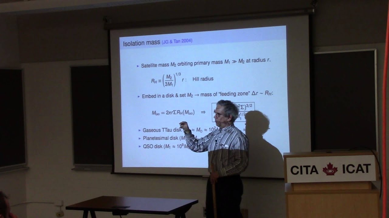
[00:14:47]So say say we have a sort like oscillating star. We have usually a lot of different pesos here. Uh we can we already know okay the diff the space in between adjacent radio order is we call large separation data new. uh we can define some small separation like say the closest let's say this one delta new 02 which is the spacing between the closed the closest L equ= 2 and I equ=0 modes uh we can define the delta new01 which is the distance between L equ=0 mode and the middle line or the two L equ= 1 mode here this uh dotted line here uh so um usually people define the separate small separation ratios like the small separation divided by the much separation to to get rid of all this global cell parameter effect and use this ratios like R01, R10 or R02. Um so this kind of ratios uh can be used to infer the interior especially the core properties or the um uh and as I can show here here are three the three uh R ratios here for this kind of uh solar type star like J star um you can see this R01 R10 this line there are some wiggles uh actually this periodicity in this R0 ratios um uh actually this multip 01 ratios is closely related to the the glitch features in the in the star and for example uh data data mu01 has been used to infer the base of the comat envelope in the solar type stars uh in in Roxburg and also uh the data uh data new02 has been used to infer the core uh properties like especially sound speed gradient and on the right we have an also data new01 uh which is uh from a model for Uranus uh from a recent paper.

[00:16:43]So actually this periodicity or this in this detail 01 uh is closely related to the core signatures because this model of Uranus has a solid core which the song cannot penetrate. So essent essentially if you do a for transform of this diagram you get a peak which closely related to the core signature.

[00:17:06]Um okay so we this this is very nice we can use combination of frequencies or small separations to infer the st interior uh but to better show the glitch features in the song or in the star uh let's do some engineering to this famous uh uh chain supermarket in the US maybe not so not so famous here in the Europe uh so after some engineering we have a structure set structure for solar type star for the f type star for all for the AB Bo type stars. Uh the red regions are the convective zone. Um so we can see for thor type starts. Okay. We have a convective envelope. We have a heliumization zone which shown here in the here uh in for the gamma. Uh we have the bottom the convective envelope here.

[00:17:55]uh for the massive or intermediate or massive star we have a conventive core uh where where the conventive core boundary can also act as a feature to create uh generate glitches. So basically this uh glitch features can be uh can act as some kind of localized scattering potential uh which will generate your oscilly component your frequency all your in your period just like what what we show here in this diagram. Um so we can have acoustic glitch or buoyancy glitch. Okay. So to study this uh we can use some techniques in quantum mechanics. Uh let's say we have some incident wave from left hand side which is propagating from left to right. And uh and then um we also have some localized potential let's let's say acoustic potential or a buoyancy potential. uh so actually the total wave function and r is the sum of the incident wave and the scattered wave. So the incident wave uh satisfies the homogeneous wave equation and the total uh wave function signifies the inhomogeneous wave equation with the potential on the right hand side and it is why known that this equation can be solved by using green function. uh if we replace the right hand side by data function and then your final solution will be the incident wave plus uh the convolution or your potential with your green function here. So okay we arrive at this expression we can give you this wave function here and r of course this is the integral equation for s uh you can see s is here s is also in the integral so so why bother so we are making things worse uh actually this equation can be discretized and solved by a matrix method or you can approximate this by using the bone approximation or bone series so essentially you are replacing this fi this side with this side you plug this whole equation into this again again again and you get this series and this is a very commonly used um approximations like born approximations let's say okay this is basically what you have inside is on the right hand side here now for the Android we have POS and GO for acoustic waves uh we have very similar equation another kind of like shinger types equation we have a potential here V we call it acoustic potential uh for granted wave we have a buoyancy potential. This is very similar. Um so again we can use the green function um like a G here. Uh we can do the convolution. We can get our final solution which is very very essentially the same as and this equation. Um so but before we do this we need to uh carefully convert our variables. Let's say for the acoustic wave we need to our x coordinate is is just the acoustic radius acoustic depth.

[00:20:50]And for the G mode we our X coordinate is the buoyancy radius. Um but but this is very nice this is very very nice analogy you can you can solve this um very right very using this grint function. Um so after after we get this solution uh ignore all of this just focus on this uh rectangle here rectangular here uh we can do some astoic analysis for this solution and uh we can write down the solution and the sign function and get this phase shift delta and this phase shift is directly related to the small separation delta new 02 or you can say 01 also um so essentially we can have a closed expression for the small separation uh so in rober use this b approximation for alco 02 uh also al three there's two small separations which are very nice uh agreement between the pro the bone approximation and the the the exact numerical values and also this is much better than the normally used as solution for data zero data new 02 which is just the the integral of the sun speed gradient Um okay so what if uh the glitch feature is large uh so people instal technology usually uh solve this by connecting wave solution in different cavities. Um let's say okay we have normally in the star we usually have a go per cavity which is uh essentially inside this brunt of vasellar frequency uh squared and we have the p mode cavity we have some abence zone between and the solution inside the cavity if it's away from the turning points are essentially sign and cosiness if they are close to turning points like just here and here they are essentially the every functions every type solutions um and in the evolution zone which the solution is essentially exponentially decreasing function. Uh so we can essentially connect these two uh solutions and get our uh final oscillation uh frequency expressions. Um okay so this has been done for subgiants or right giants on the left we have two cavities for right giants or subgiants we have G cavity or B cavity and on the right there are three cavities because this is a red giant undergoing helium flash because the helium flash is offcentered we have this additional convective convection zone here so which separates the original GM mode cavity so we have two three cavities here uh you can connect the solution in the three cavities and get your again get Agon function or AEN frequency uh relations but the AEN but the power but the authority spectra for this kind of flashing star is more complicated of course. Um so of course uh uh you can essentially uh extend this all the way to n cavities as large number as you want as we want. Uh this been done for by uh by pong and teata.

[00:23:49]Uh so you so we have encounties and each interface we have some uh transmissive and reflective coefficients.

[00:23:58]Um and also for um for the cases if we have magic fields and rotation this a recent work by Lucas if we have uh a star let's say a data a gamma door star we have count core and radial envelope uh and it's rotating and in the in the in the radial envelope here we have the gr inertial with the grual grant wave I'll say inertial grant wave g the gavity which is described by the whole function and inside the com core uh we have the the pure inertial mode which I essentially have this kind of brine solutions. Um you can connect these two solution and interface and work out your pure spacing and which will generate a dip in your pure spacing and pure diagrams. And by the way, this is the pure inertial modes inside the connective core. Um, which are usually described by two quantum numbers and and also this pure inertial modes have a singularity belt which is along the direction of the described by the spin parameter here. Um, okay. So in some in some other stars like STB star we have some structure well structured uh envelope bant and core. uh let's say if we plow the brunt frequency bras frequency which is here we usually have some bump or a spike due to this structure or the chemical discontinuities uh sometimes if the the mode uh has a node near near this bump the mode can be trapped uh and the two bottom plots uh are showing this kind of weight waiting functions like whether the moles are concentrated by this single u uh single uh region And um and for this this is tramped mode this is the normal mode. Um so actually we can also connect solutions uh let's say uh migrator and the paper which connects solutions on both side on both sides of the glitch in the brown frequency profile and get your uh buoy buoy glitch or buoy frequency um relations. Um okay so uh I'm sorry about all these equations but now I'm going to do some engineering to the right hand side of this equation. Uh we add a source term and I mentioned I can this source term can be a title force uh oh sorry um okay let's say this title force can be a harmonic forcing from the companion star which is a sum of the opto forcing which is integger which is n times opto frequency. Um and this um so basically we we have this equation.

[00:26:35]Uh we can solve this equation by simply expand our solution as a sum of a functions from adabatic functions with some slowly varying amplitude C. So around and this equation for C which has this very uh how this closed analytical form. Uh so we have this totally false mode. We have the amplitudes predicted.

[00:26:59]uh we have the predicted amplitude also the faces uh so of course we have a lot of uh harb observed by capture or test which we can apply this uh to the title forced waves um so now the we can do some engineering to the right hand side now the right hand side is uh a nonlinear term uh let's say we keep the quadratic ninear term here so we do the similar stuff uh expansion of the solution and the functions and we slowly varying amplitude Q and now you work out you plug this to plug in this to this and you get this amp amplitude equation you for three mode coupling case uh in this three mode resonance three mode coupling case where we have this frequency relations here and all this equation it's relatively simple ODS and uh it's only the only difficult part is just the the three more coupling coefficient term here um but this is essentially depends on uh the integral of three spherical harmonics which will naturally give you some selection rules because only uh um only in this case you can get a nonzero coupling coefficient. Uh by the way this three coupling is is ubiquitous. uh uh you may uh okay so um let's say um you may already experience some stream coupling here because uh I I didn't realize this laser pointer is green uh so but anyway if you have been doing stargazing you have already held some firsthand experience because the red laser or infrared laser is easy to make and usually to generate a green laser you need some ner crystal and uses the second harmonic generation. This is kind of three mode coupling. Um so basically uh what what is green laser is the result of three mode coupling here.

[00:28:56]Um so this is a case of direct resonance which means we have two low frequencies here. Um generate a third frequency or higher frequency a third frequency which are higher. Um so we have some observations in the three mode coupling.

[00:29:12]This is called direct resonance. Uh these are like three three P modes coupling to each other. Uh if you or if you plot the amplitudes of these two modes A and B and also the C you can see this signify this very nice relation. Uh we already scaling depends on your coupling coefficient also the resonance uh or your D-tuning in the resonance.

[00:29:35]uh so we also have some uh evidence uh of three mode coupling in SDB stars or subd stars as well. So uh another case for three more coupling is called parametric resonance.

[00:29:47]In this case we have one mode here which is unstable it's driven and then we have two low frequency modes uh satisfy this relation. Uh so let's say this is a power spectra from a data scooy star. We only see one p mode. we didn't see omega A omega B here because they are very very high LG G mode somewhere here which are are not visible so the the best uh daughter mode pair is actually with L from 50 to 200 for this case so this is not possible to see actually um so this parametric resonance can act as a amplitude saturation mechanism uh to saturate the amplitude of of of this mode uh so Yum Lee has calculated the saturation amplitude for SPB starly posted in B star. Uh we can we use some very reasonable luminosity probabations and Jimski calculated this for data school star POS and also there are some other papers uh uh talking about the different mode behavior when this remote couple to each other. So uh indeed in this remote coupling case uh this mode behavior can be very different they can be chaotic. This is the mode amplitudes or wound the mode. Uh it can be in limit cycles. Uh depending on essentially two parameter one is a d tuning like how far away this is from the perfect resonance and the second is the the damping rate ratio which is essentially the damping rate of daughter divided by damping of the parent. So we can have different type of mode behavior. We can even have chaotic or unbounded or pure doubling all the way um to chaos. So you may seen this kind of peration diagram before. uh this is the peak amplitude of the mode and this is uh an a parameter the damping rate ratio which I mentioned before by slowly changing your damping rate uh like essentially daughter divided by parent you can the mode uh the system can have different behavior you can have period doubling period 2 pure four pure eight all the way to chaos and inside the chaotic region you may have periodic region um so now we can do some engineering to the right hand side now we keep the cubic nonlinearity term. Uh now okay so we have now this house formal coupling essentially we have this frequency relation here. Um this can be applied to the L equal to one triplet like rotational splitted triplets because because this we naturally have this resonance condition for the frequency in the splittings and in this case the mode behavior depends again on the duning like the tuning data new also on the damping rate. Um so actually there are three different regimes for this kind of formal coupling. Uh the first regime is kind of stable regime where the detune is very very small. Uh in in this case we have stable amplitudes. In the second case if the d tuning is approximately the same and the damping rates uh the system will undergo this kind of modulation and this modulation in amplitude and frequency. uh the modulation time scale uh essentially one over datanu one over the d-tuning in the frequency and finally we have the third region which is non reg essentially if the d tuning is very very large essentially we have three individual modes um I'm sorry about some of the text um so um actually after talking about three mode for more coupling we can do a little bit better um like we can write down the nonlinear wave honing uh we have linear wave and nonlinear uh part and linear part the the interaction part the wave interaction Hamiltonian which including a three wave interaction four wave interactions uh so we can write down the famous Hamilton equation we all learned it from classical mechanics um if you uh use some variable transformation you can convert this two equation to one equation which is essentially this equation uh uh and a is the wave amplitude um so we have if you have some Hamiltonian you already have this equation of motion for your wave amplitude. Um so for uh so this is called the kinetic kinetic equation for wave amplitude. Um so if we square your amplitude ampl your wave amplitude you get this uh wave action or wave essentially wave energy very very closely related you you can get this equation for wave action n here which is uh described how the waves interact with each other uh this equation is in for space so it's it's a different wave vectors um so why are we doing this because if we do this for a large sample of waves So we can do some if we assume the waves have random faces we can do some ensemble averaging. Um we can find a stationary solution for this wave action a. If we if we assume that the wave action a scales with the frequency of wave vector to some kind of power law.

[00:34:45]Um after we get a solution we may find the stationary the let's say the stationary power law for a and b. So we we will have a stationary slope in the power spectra. So this can be done for the ocean gravity waves. So in the ocean gravity waves we essentially this ocean ground waves are generated by the wind on the surface and also the tidal uh force. So uh the the wave interaction is essentially the three-wave interaction is the dominant mechanism which can uh generate your equilibrium power spectrum. So actually there is a universal power law uh spectra for the internal grad wave in the ocean. Uh let's say this is the uh the power spectra and function of wave vector or wave number vertical wave numbers uh with some slope. So this spectra is called the gith monk spectrum. Uh so actually this spectrum uh ignore or ignore all this text I'm sorry uh just focus on here. uh this power spectra has a slope of minus four. If we and the high uh wavelength high wave vector tail essentially the essentially the power index is four. The exponential index is minus four here and this uh all this uh previous uh all this previous calculation this kind of calculation give you um it's really this should be minus minus 3.7 minus 3.7 which is very close to the observer spectra. So essentially we can have uh a framework to calculate your power spectral slope in your gravity waves for the ocean ground waves. Okay. So um now I'm um stepping outside uh our subject and talk about a little bit about mechanical engineering. Uh let's say we have some kind of optimiz optimization problem. It's called a topology optimization. Um so we have a working domain which is essentially a 2D beam.

[00:36:44]We want to um do some optimization. We want to maximize the structure stiffness. We want to keep the volume half. We can keep half the volume just like this or like this. And then we uh maximize the structure stiffness. We also maximize the the J's natural frequency.

[00:37:06]Um so so this is one of the the fundamental mode of this uh beam. Uh so if you if you solve this optimization problem um you can find your your optimal structure for this 2D beam. So I wish we could do this for the star. So but unfortunately probably it's very difficult. Okay. So uh now I have um talked all about this uh different uh mathematical techniques. Now I'm going to talk about some other things like this is one of the famous article written by Nick Trafferson. Um you may heard you may heard about him because he has a very famous book on spectrum methods. Um he has some favorite egg value problems. uh for example uh one let's say maybe the first one is the the bay of founding in Canada which give you a 16 meter tide 16 meter tide uh war that is world record um and the second so any regular panting you see in nature probably maybe the cloud stripes or maybe some ripples on the sand is some results of the egg value problem because it it is this aen mode which grows faster than others. Then finally how uh this essentially the leftover of the competition.

[00:38:27]Um this is another uh egging value problem. Uh and finally going to talk about a joke by by Chandra. Uh so this is a figure generated by OK GPT. Uh so this is uh since this is a birthday party uh held by Kip Sworn uh one of the the Nobel laureate in Kotech and and Chandra was visiting Kekch and uh Keon was insist in insisting on hosting on host host this birthday party for him and Chandra is is sitting in the center here. We have some other people here like Saul um Cholo Kosski which is a famous numerical relativity expert if you have heard have used the rotating curl black holes. Uh we also have the William press which which is a the author of the numerical recipes. Um so so basically um they are sitting just in a dark basement and and then keeps one keep was trying to keep the conversation going and and then Chandra said let me tell a joke. Um okay go how can we divide 16 lumps of sugar um into three teacups and each having a nonzero out number of lumps we have three tea cups 16 lumps of sugar um okay so uh there silence and then saw ventured and said okay we can this is probably not possible and then uh okay because because the sum of three odd numbers is always odd Um and then Chandra said, "Not at all. You can put one in the first cup, one in the second cup, and 14 in the last cup." And and they said back triumphantly. And then Saul said, "Okay, 14 is not 14 is even number." And then Chandra said, "Okay, um I would say 14 is an ex exceedingly odd number of lumps to put in a single cup of tea." So uh so I will uh leave this and uh thank you so much for your attention.

[00:40:31][Applause] Thanks Raul. Um I think if we had prices which we I guess should establish roles for the next academic year, I think you would have high chance of winning one for the largest number of equations per square centimeter per second. I'm I'm very sorry. I'm I I should do better than that. But uh thanks for the beautiful M. Uh questions. Time for questions.

[00:41:08]Uh hi Shiao, thank you for your talk. Uh I have a couple of questions, but I guess I stick to one. Um uh so as far as I understand when you use the linear force operator you use it to get linear terms and to get the stability of solutions as well as the frequencies and uh I I would like to know your opinion about using nonlinear force operators. Do you use the same kind of thinking about it or is it more complex? Yeah, you can work out the similar uh stability condition by by plugging into your exponential solution and check out the values and so you use it for stability and the I can again function yes we have you can you can hold the I didn't show it here for the three more coupling for the force three mode coupling you can have stability for this one more solution or three mode solution uh I mean the technique very similar to the the normal three more coupling equation you question. How do you select that at which order to stop? Which to stop? Yes.

[00:42:18]Oh, I stop already and quadratic or cubic term. So I work uh for three more coupling of course you stop and quadratic nonlinear terms. You you just ignore all the rest. For formal coupling you only I only concentrate on the three more coupling or on the third order nonlinear terms. So um so essentially you can include all of them uh it will make your mod network large um uh um okay so this is basically uh this is basically the wave turbulence equation I shown which you can but you don't want so all this equation you want to do some averaging in the end [Music] um so did I answer your on. Yeah, I think so. Yeah.

[00:43:11]Okay, there's still time for questions.

[00:43:16]Hi Joe, thanks for a lot of really fun information. I was really interested in the beginning of your talk with these line integrals where you used you showed their application for um photodnamic modeling and also the modeling of the like spot module not the the net tooidal flux on your star. I was wondering if you can apply this to the case of the modulated observed amplitude of pulsations when you have an eclipsing binary. So right you you normally you have your your disc and then when you have the eclipsing binary you preferentially block out parts of the star therefore modulating the yeah I'm well simply um well while if you replace this limit limiting law by sparkle harmonics or some kind of combination of that um I don't I I I I think you can do that I I I don't know uh but I I think you can do that because you you should be able to do this in two ways, right? So, you have the your line integral describing the surface and your limb darkening and then you have the original that's acting as a filter for the original spherical harmonics that are underneath it. So, you should be able to get a time dependent formulation of what the mode visibilities are for an arbitrary set of modes. Yeah, this is doable I think. Yes, that's a very good point. That would be really helpful.

[00:44:40]Yeah, I don't think anybody can try that. Yes. Do you have time? I don't know.

[00:44:47]Thank you. Let's see.

[00:44:50]Still have time for questions. I have a I'll have an very annoying one for you, I guess. Uh I'm an observer.

[00:45:01]Me too. I Yes, you're also an observer but doing a lot of theory. Um so uh fine too. How can we meet and start talking same language?

[00:45:12]For example, when you speak about nonlinear mode coupling, you have this elegant mathematical solution to the problem and then you say, okay, we kind of observe this in in stars as well.

[00:45:24]What do I learn from that? Uh you learn about the essentially the mode damping mode driving rates. Uh I see what I what do what do you learn about the evolution of stars from that or interior structure or something about stars in physical terms?

[00:45:47]Um well I I think uh one of the implication you can think from the three remote coupling uh if you see some kind of three remote coupling here you may have observed frequency and faces you can have this kind of inference on this kind of coupling coefficient which directly give you this kind of uh d-tuning and uh damping rates like the imaginary parts for the frequency the d-tuning uh is evolutionary very dependent. Of course you for different type of star your mode density will be different. You may have very strong resonance for later for later evolutary stages if your most uh dense for the early star you may have less strong uh I should say uh resonance and this will this will change your coupling coefficient and then eventually change your relation between your daughter moles and parent moles here. Um so it says if you plot this kind of observe the relation you may have different kind of scaling uh we need to scale this red line to the blank line so you may have different scaling which is kind of like a edge indicator I mean I should say it's a very very slow viring functional age but u uh I think in principle you can have some you can have a handle on on the age possible um of damping risk is it also of course depends on the the st the illuminary stage of the star. Um um and of course the the version three mode coupled to each other they settle into a stationary solution and this solution is also age dependent. Um so you may have some observed modes with some fixed amplitudes maybe have lower amplitudes uh if the resonance is stronger higher amplitude if it's not so strong. We haven't been uh people haven't seen this in data school star for like older uh data school star or younger data school stars uh I think um but but is it's a little bit difficult but uh but you can link this to observations uh if you work hard enough yes and this is something we can learn only from the observations theory of nonlinear mode coupling we cannot learn these things from just normal modes the normal most like well if we ignore the nonlinear coupling for example in our modeling how how wrong can we be you ignore the normal modes you only can okay if you get rid of all this combination frequency you work only on the individual frequencies um um I think most cases should be fine uh except for the strong cases where the frequency shift due to mode coupling will be strong um um well we have been doing this all along right formology. So if it's not um I should say it's okay to to do that in most cases. Um okay yes there is still time for questions.

[00:49:00]So when you were discussing about the the solution of the of the linear force equation and you add the magnetic field as a source term do you get a different solution as when you deal with the MHD equations that's to say you get also magnet acoustic modes and alen oh I did not I did not answer the mfield and s term but only the probabation term to the linear operator L. So it's a it's a a probabative approach and it's there's no resonance to wave. So you you now get that here um by this approach. Um so this is very simplified. So it's a very approximating way of or calculating frequency shifts. Um so is it just more to separate the um the generacy of of P modes? Yes, I mean you can uh this part methods you can I I didn't show it here but uh uh your um your frequency shapes can be written uh for a different m and you can work out the the so the probabation of the linear operator and the inner product this this this kind of term can be written and the matrix you I mean Vincent also yellow is working on this kind of thing and um so I mean this what I'm showing here are rotationally dominated as simple perturbation treatment. I think yeah we still have time maybe one more quick question from me. Um so to be honest you you lost me a little bit halfway through the talk.

[00:50:54]Maybe the answer was towards the end of the talk to my question. But um what I know about 4D star is that you know it's about doing stars in three spatial dimensions and one time dimension.

[00:51:10]So what's what ingredient in your talk uh reflects on the upgrade from 1D to 3D or 4D?

[00:51:22]Yeah, I mean um well uh there we have 1D oscillation code, 2D oscillation code uh by assuming the five uh and muscle angle is always the symmetry is keep is kept.

[00:51:35]Um but of course you can relax you can have the 3D. So in in mechanical engineering people using finan methods usually to structure to study the agon mode structure they call it a model analysis st study the stability of this agon frequency of this beam or different kind of structures. Um um but this uh or other other kind of numerical method like fin volume or or special element you can just people are not so um I should say um dedicated to apply this method to station equations.

[00:52:13]uh um so as uh I mean in principle you can do this kind of optimization by um by by work out on a 2D domain or 3D domain um um for the start just uh uh we need some knowledge from other fields I should say or from numerical or CFD.

[00:52:40]Okay, last chance to ask a question. If not, then let's thank J again. Thank you.

[00:52:54]Thanks for coming. See you next week.