

![Diskrete Fourier Transformation [DFT] | Signale und Systeme](https://i.ytimg.com/vi_webp/TVKtwf1gJSs/maxresdefault.webp)







![[WEBINAR] Gestão, Diagnóstico e Contestação do FAP 2026](https://i.ytimg.com/vi/6e-dxZOf2JE/maxresdefault.jpg)






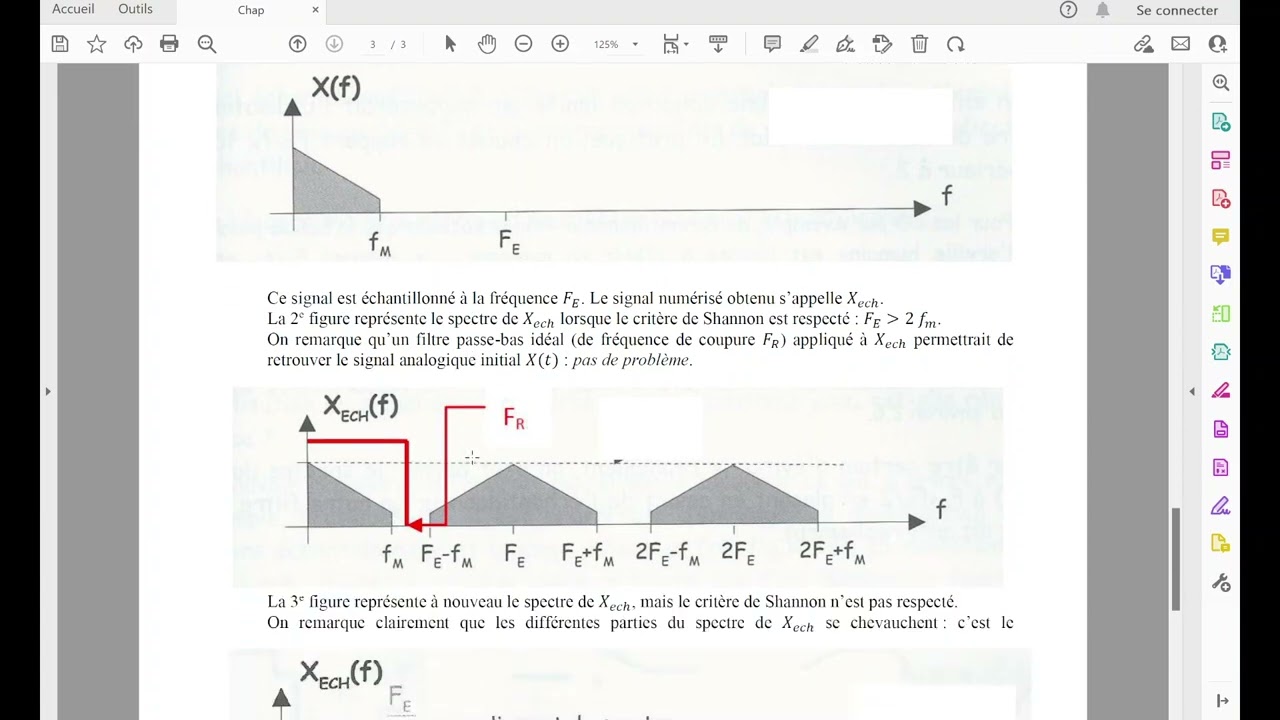
The Lomb-Scargle periodogram is a statistical method that converts time-series measurements (such as stellar brightness over time) into power measurements at different frequencies, enabling astronomers to detect and characterize periodic signals in astrophysical data; this technique works by fitting sinusoidal functions to the data at various frequencies and calculating the chi-squared statistic to determine which frequencies contain significant power, ultimately helping identify the period of astrophysical phenomena like variable stars or eclipsing binaries.
Lomb-Scargle Periodogram Explained for Astronomy Data Analysis
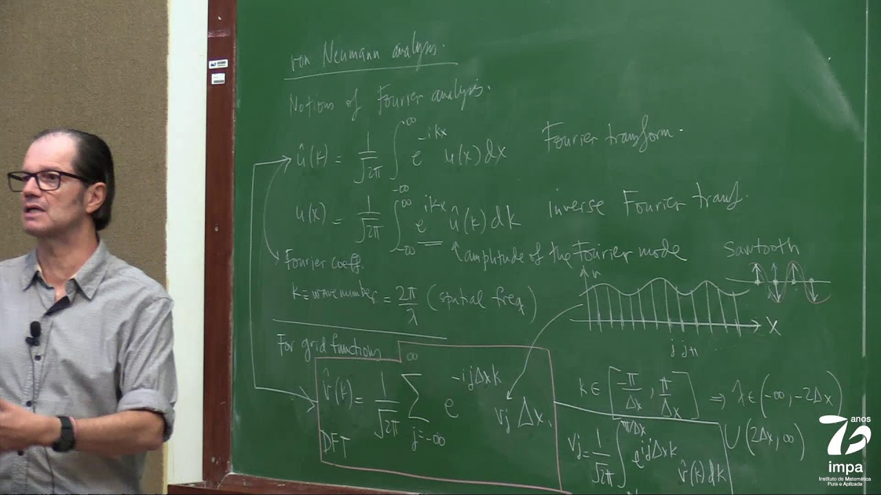
Added:Basic concepts of Fourier analysis and spectral decomposition, such as the Discrete Fourier Transform (DFT).
The challenges of unevenly spaced time-series data, which is typical in observational astronomy due to day/night cycles and weather.
Fundamentals of Python programming, specifically using scientific libraries like NumPy, SciPy, and Matplotlib.
Basic astronomical concepts of periodic phenomena, such as stellar pulsations, binary star orbits, or exoplanetary transits.
Calculating False Alarm Probability (FAP) to statistically evaluate the significance of detected periodogram peaks.
Phase-folding time-series data using the detected period to reconstruct and visualize light curves.
Exploring alternative period-finding algorithms, such as the Box Least Squares (BLS) method for detecting shallow exoplanetary transits.
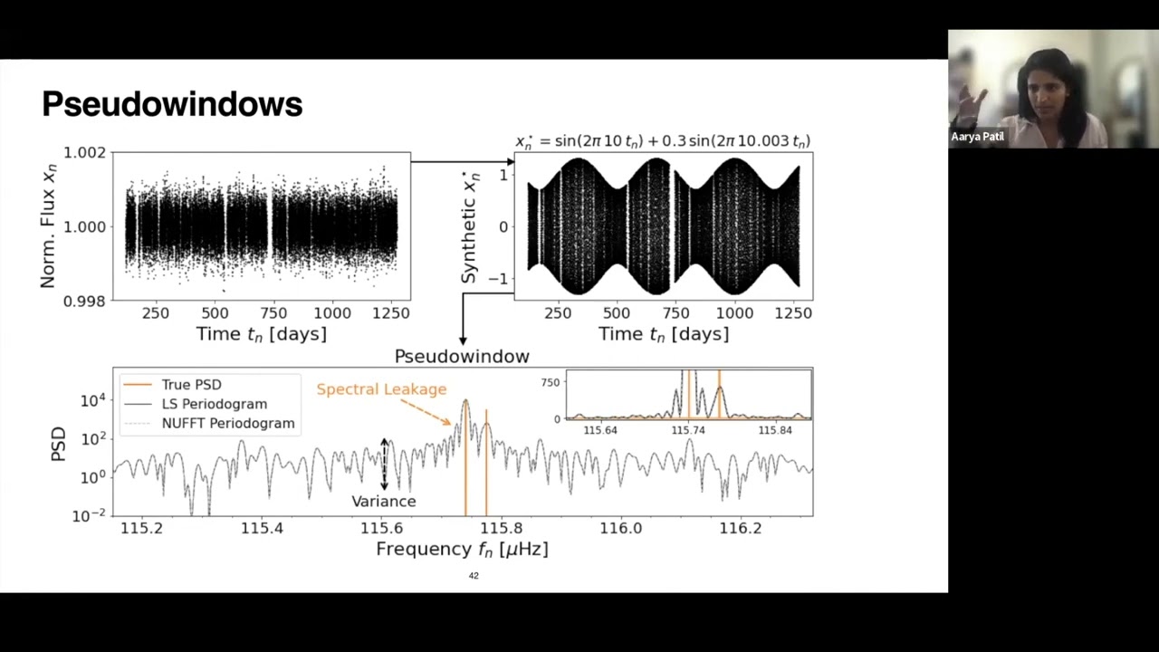
Mitigating the effects of red noise, aliases, and window functions on spectral analysis in astronomical datasets.
4K views103likes28:15Original Release: 2023-08-15
hi this is robert quimby and i'm going to tell you about the lone scargle periodogram so as an astronomer you may go out and measure a signal maybe the brightness of a star over some time and you may look at the signal and notice that it's not constant that there's actually some fluctuations in signal over time you might want to quantify those fluctuations and see if this is a periodic signal so what you want to do is go from the magnitude of the star over time to the power in each frequency so one way to do this is to calculate the lone scale periodogram and that will give you this information here frequency the power versus frequency and then using this you can go on to figure out what the period of the signal is so in this tutorial we're going to begin by just reviewing fourier decomposition remind you that you can take any periodic signal and you can represent that with the sum of a series of sine and cosine terms we're going to actually do that we're going to go through this exercise and create a signal just using sine and cosine terms and then we're going to do the reverse process we're going to take the signal we've generated and we're going to deconstruct it and find what the what the amplitudes of each one of those sinusoidal terms is this is essentially what the lone skeletal periodogram does and so we're going to actually then use the lone score periodogram to find the period of a real astrophysical signal as always this is going to be just a quick introduction to the topic if you want to know more there is a nice paper by jake vander plass that will go into much more detail on this i suggest you check that out so hopefully if you've seen this before in your math classes you can take any periodic function and you can represent it as the sum of cosine and sine terms each one of these is going to have a slightly different frequency and they're going to have different amplitudes but by adding up these sine and cosine terms you can represent any arbitrary periodic function so for example we can look at the decomposition of triangle waves so triangle wave is something that starts off and goes straight up and then straight down and straight up and then straight down like that that's a triangle width so it's similar to a sine wave but it's not as curvy so how do we go from these curvy sine waves to these linear changes well all we have to do is actually just take the sine terms we don't even need the cosine terms find the appropriate amplitudes for the appropriate frequencies add them all together and we'll get a triangle wave so we can go ahead and code this up in python so what we're going to do is we're going to just add each one of these sine waves uh in this list we're going to keep track of that we're going to convert it to an array at the end and so we're just going to go through each one of these n terms we just need the odd terms as well so for the odd terms we're going to record the amplitude and that's just going to be minus 1 to the power of n minus 1 divided by 2 divided and that's all going to be divided by n squared so that's going to be the amplitude of each one of our sine waves we also need to record the frequency here that's just going to be n divided by p here so divided by our period and then we can create a sine wave at the appropriate frequency multiply it by the appropriate amplitude and we'll keep track of that in our components so now we can test out our function we'll just create a bunch of test times just between zero and three have a thousand different points where we'll calculate what the signal should be at each one of those so we're going to get the components for each one of those terms so we're going to give the times where we want to be calculated and we'll pick how many terms we want let's start with say two terms and then for each one of those sine waves that we're going to generate we're just going to plot them start with that so here we are so you can see the first term here it's a blue one here we've got just a nice sine wave and then the second order term is just a higher frequency sine wave with a lower amplitude so let's add another term here and you can see what's happening here so each time we add a term it has a peak at the same spot it's always going to peak right here it's always going to have a trough right here and so on and so what this is going to do is it's going to be if we add these together it's going to lift this peak up and over time these waves are going to get more and more narrow so it's going to end up giving us a very very a fine point here on our peak and a fine point on the trough and then on the sides here what we're doing is we're kind of taking out some of the curve in this here so we're subtracting a little bit here and a little bit there to make this in more of a straight line so if we actually just look at the sum of all these terms that's the wave that we want to generate here that's our signal and that's just going to be our components the sum of those and we're just going to go over axis 0 so that we we don't want to sum over time we want to keep all those times we're summing basically vertically in this plot and we'll take that signal we can plot that as well we'll make these lines black and we'll put in a boulder line we'll make a line weight three and we'll plot this and there we go so this is the line where we've generated with just three terms just three sinusoidal terms we add those together and we get this black line here and you can see what happens now is we add more terms the peak gets a little bit sharper and this line gets a little less wavy and so we get five terms we can add six terms and as we do that you can see every time we're getting more and more linear here and more and more peaked here eventually you can add a whole bunch of terms and you see what that does it gives you something that's very very close to a triangle wave and of course in the limit that we have an infinite number terms it's exactly a triangle wave but just with six terms we actually get pretty darn close to a triangle wave so we can see from these components that the the first sign we made this this blue curve here is the most important in defining this triangle wave all these other terms are they're adding to this they're making it closer and closer to a triangle wave but most of the power is actually in this first term here so let's explore that now we're going to take a look at what those amplitudes are for each one of our sine waves so again these are the bn terms we're going to keep track of that in the frequencies just going to use six terms here stick with a period of one and then we're going to add all the terms i'm going to keep track of the the even ones as well so if we have an even term we're just going to set the amplitude to zero fit odd term we're gonna set the amplitude as appropriate for a triangle wave and then we're gonna record all these amplitudes and frequencies and turn those into arrays so we can work with them so i'll run that and now what we can do is we can just make a simple plot we're going to make a bar plot here just showing for each frequency what is the amplitude and there we have it so we can see again we already knew this visually just looking at the plot but that first sine wave has a much larger amplitude than anything else uh it is important to note that some of these amplitudes are negative so that second term has a negative amplitude and then goes positive negative it's got this odd even effect here so often what we want to know is what's the power in each one of these terms not just what the the amplitude is but what's the power and so to calculate that all we need to do is we can just square each one of these terms so let's go ahead and do that again we're going to plot our frequency and now we're going to do the power so we're going to take our bn amplitudes and just square those and this will give us the power so we can see here that most of the power again is in that first term and then it decays pretty quickly after that so i'm going to put this on a log scale just to make it a little bit more visible what's going on here now you can see these other terms peaking up here but again it's a log scale now so these are much much less power in each one of these terms than in this first sine wave so hopefully this reminds you that you can take a series of sine and cosine waves and you can put them together you can make a triangle wave but that's not the case that you're usually working with in in astronomy usually you're given some signal and you want to do the reverse process you want to figure out what the power is in each one of its frequency components so let's start now with this signal so we've sampled a triangle wave at discrete points over time and what we want to do is just given these data just given this signal at these times we want to reconstruct the components of the triangle wave and we'll see if we can get exactly what we put in because we know what we put in to make this triangle wave let's see if we can recover those just given these data points here so there's different ways we can approach this problem but from what we've just motivated one way that you can think about this is that we can actually just go and try and fit sine waves of different different frequencies to these data and see how well the sine waves fit and if the sine wave is a good fit at some frequency then we can say well that frequency probably has a lot of power in this in this signal and if it's a poor fit then we can say well it there's probably not much power for that particular frequency we picked so all we have to do is pick a whole bunch of different frequencies do a fit maybe a least squares fit to figure out what the best fit amplitude and phase are and then record how well each one of those fits represents the data and then we can use that to reconstruct the amplitudes of the terms in the signal so to the data we have we have data y data points sampled at times t and all we need to do is fit a function like this we just can use any sine sine square i'm going to use a cosine here you can use a sine if you want there are just a difference of a phase shift and we're just by adding these terms together we can fit for the amplitudes and phases here and figure out what the best fit values are and then ultimately determine if that's a good fit to the data so if you look at the way i've set this problem up here you you may immediately notice that the two parameters we have a and in phi here are not linear in this equation so we could use some non-linear least squares fitting to figure out what these these terms are but it turns out there's a nice trig identity that will allow us to do just straight linearly squares fitting so all we have to do is just recast this equation in a form that is linear in a and phi and the way to do that is with a trig identity so there's an identity that's a cosine of some angle plus some phase is just equal to the cosine of that angle plus the sine of that angle with some different weights than we started out with so this is very handy to know all we have to do to fit the problem at hand is we make the substitution that theta is is equal to 2 pi times the frequency times the time and then note that we can recover what we want we want the amplitude and the phase information for each one of the models that we're going to fit and we can get those in terms of the b and c values that we're going to actually fit for so the a amplitude is just the hypotenuse of b and c and the phase phi is just the arc tangent of c over b so with this trig identity in place we can go ahead and set up our equations for a least square solution so again we have our observed data points our y's and we just set that up in a column matrix and then we have what we're going to calculate we're going to define y is going to be equal to b cosine theta plus c sine theta so we have one just cosine and sine terms for each given frequency at each time multiplied by our amplitudes b and c and then we can fit for b and c so let's go ahead and code this up in python first thing we should do is figure out what frequencies do we want to test we can test any frequencies we want but we kind of already know we should just be testing integers because that's how we set up the problem so we'll just make it easy just do numpy a range of different 11 different values we want to start with one so we're going to add 1 to that and then we'll set up our y matrix so this is again the signal at each observed time so that's just going to be the value for value in our signal and again i put it in square brackets here because we want a list of lists so we can make a numpy column matrix and then we'll set up all the amplitudes that we're going to fit for the phases we're going to fit for and then for each frequency we're going to test we're going to set up our thetas right for each time and then we're going to create our x matrix so we can solve y equals x times p and so this is the matrix that has the cosine theta and the sine theta terms for each theta in thetas so then we solve this as always we do our matrix algebra here it's a solve for p and then from p we can extract the parameters b and c that we just fit for and then we can convert those to a and phi using those trig identities that we just discussed and so at the end of this we're just going to take those a values convert them into numpy arrays and the fives and convert those to numpy arrays and we'll have our best fit values so i'm going to run this and it runs pretty quick and so now for each one of the frequencies we tested we have the best fit amplitude and phase so let's make a plot now to see what this looks like let's first start with a bar plot like we showed before just the frequencies that we know are important and the amplitudes that we assigned when we can when we created that triangular wave so it looks like this we saw this before and now let's add to this a bar plot with the frequencies we've tested and the amplitudes that we've found the best fit amplitudes squared and we're going to go ahead and normalize these to the maximum just so we get one here in the first term i'm going to plot this with just hatches with red hashes so we can overlay that and there we are so you can see just by going through and testing these different frequencies we've actually done a great job of recovering the power in the model that we constructed in fact there are identical matches up to the scaling factor we have identical values in each one of these odd terms and we have a little bit of power in these even terms you'll notice creeping up here but you know remember this is a log scale here this is 10 to the minus 29 here so there's very very little power that we're detecting in these and so otherwise we've actually succeeded in taking the signal just the measured values over time and converting that back into power at each frequency so this is very close to what the lump scar goal process is but there is actually one additional twist so here we're just fitting and we're showing what the best fit parameters are for the amplitudes squared for each one of the sine waves we've tested we didn't say anything about how well they fit so that's actually of one further step that is done in the lone scale process and that is for each fit that you run you actually calculate a chi-squared value and you use that to determine the relative power in each one of those frequencies so we're going to go ahead and do this we're going to set up for chi-squared fitting so we're going to have a model which is just those two terms the amplitude and the phi and the model again is just the amplitude times cosine of our angle plus some phase phi and then you evaluate the chi-square all we have to do is calculate the predicted model values at each one of these times and then compare that to the values that we actually observe looking at the residual squaring that and taking the sum of the square of the residuals as our chi-square value if we did have uncertainties we could also divide these values here this residual by the uncertainties but in this test case at least there's no uncertainty so we're not going to worry about that we should define our chi-square this way and now we can test this out so for each one of these frequencies that we've done our fitting at we can go ahead and calculate with what the chi squared is we just have to give it the best fit model parameters at each one of those steps so this is the a the i a value and the ith phi value those are our parameters our best fit parameters and these are the times that we sample that and the frequencies at that ith bin and the signal that was observed so we'll append all those chi-square values and convert it into a numpy array we have our chi-squares now so the last thing we need to do is to convert these chi-squared values that we've calculated into a power and the way we can do this is we can compare these chi-squared values to the chi-square we would get for a constant signal so that would be equivalent to taking these models that we fit and just setting all the amplitudes to zero just we have a constant value over time but our models have more flexibility in them and so that means that these models should always do better than the simple model of just a constant signal over time so by comparing against this kind of reference model here we can get an idea for the power in each one of our amplitudes so to define this reference chi-squared value we're just going to calculate a chi-squared for a constant so which is just the numpy sum of the squares of the residuals that's our signal minus this constant term which i'm going to set to numpy mean of our signal and that's all going to be squared so that's our reference chi squared value and then to calculate the power we just take our reference value and subtract off the values we can we calculate for our best fits and there's different choices of how you can kind of normalize this here our popular choice is to just divide by the chi-squared 0 by this reference chi squared value and that will give you the power for each one of frequencies so let's go back to this plot that we had before where we're looking at different frequencies and looking at the power in each one of those so far we've not actually been plotting the power which is plotting the amplitudes squared so the blue is the original and the red is our best fits let's see what happens when we add the chi-square to this we're going to plot this with hashes going the other way in black and there we have it so other than a tiny scaling factor you can see that we've reproduced the amplitudes in each one of those frequencies with power and now this chi-squared value actually we have zeros here in the even terms which is good so we now have what's called the loamscargo periodogram for this signal the power at each frequency so that's great for test data why don't we try something real so this is real data in this vera star file for a target in the sky we've got the modified julian dates magnitudes uncertainties and a photometry flag there for this and so we're going to just pull out those times and the signal and plot those and this is what we get so this is the magnitude of a star over some time and you can see there's some fluctuations in here and if we actually zoomed in we can see that this isn't just random noise here let's see go to uh seven four two four and five seven four two eight zoom in a bit here you can see that there is actually a signal going up and down and up and down here maybe a few times per day so let's now figure out what the period of this is just based on these data that we have to make things a little bit easier i'm just going to start by subtracting off the average value of the magnitude okay so now we get numbers that are closer to zero here and then all we have to do is essentially just what we did before we start by choosing what frequencies we want to evaluate the power out and for this time let's do a whole bunch of frequencies we'll do the numpy line space and we'll span the range we think is important it looks like it's there's variations over at least once per day maybe up to 15 times per day and so let's pick a thousand values evenly spaced between those two and we'll test the power in each one of those frequencies so then we'll set up our y matrix just like we did before it's a call matrix we're going to record the amplitude squared and the chi chi-squared values just we have both to work with if we want to compare those later and then for each frequency we're going to do the chi-squared fits we can find the best fit parameters we're going to convert those into our amplitude and our phases and then find the chi-square for that amplitude and phase and record that and once we've done all this for each frequency we're going to have our baseline case here which is just a constant signal so we'll look at the chi-square for constant signal and we'll calculate the power the ohms cargo power in each one of these frequencies so we'll run through that and now we can plot the power in each one of these frequencies so instead of the simple bar graphs we did previously now we have a thousand values so we're just doing a regular line plot here and you can see there is clear contribution from a number of different frequencies in this signal those all add up together and produce the signal we observe so this is actually norm's cargo periodogram so that shows you how the lone scarves periodogram is actually calculated you don't actually have to do all these steps that we did before you can just use the version of loms cargo that's built into astro pi so in astro pi time series there is a lone scargle object that we can import and then we can use these with the data and it's it's all an astro pi so it works nicely with astro pi units we can now define our times to be in days uh and our magnitudes to be in magnitudes and we can use these and we can calculate what the lumescargo periodogram is for these data just pass up the times and the magnets and we'll give us a little score periodogram if we want the power for this we can just say okay calculate the power and we tell it what frequencies we want to be calculated at and we can specify units here so we if we specify units here we have to specify units here so i'm just going to divide this by u dot day and then get rid of that inner one and there we go so you can see this is virtually identical to what we did before because that's essentially how this is coded up in mom's car with some minor differences you should also add that in loom scargle this is defined by astro pi it also allows you to give the uncertainties in your measurements so you can put that in there also one of the key things in this process is picking what those frequencies are and lumpscargo has some tools built into to automatically pick some for you which may be a good place to start at least you might want to change them after you've seen what you got but you can always start with them so we can use the lumscargo auto power function and that'll actually pick the frequencies for us and calculate the power at each one of those and so that's what that looks like so again very similar to what we just had it's just now we're using these uncertainties to weight the fitting and we're calculating the frequencies that were automatically chosen so we now know the power in each one of these frequencies that we've tested and we can see which ones have the most power but what you might be interested in is knowing what the period of this object is what's the period in this signal we have to be a little bit careful in interpreting the periodogram to get the period we can just start with the peak frequency the frequency with the most power in it but we have to remember that when we're doing this fitting when we're doing lum's cargo we're fitting sine waves sinusoids to the data and sinusoids have an up term and a down term and then go back to where they started your signal may have more ups and downs than a sine wave does in each period and so because of that you have to have some knowledge of what your astrophysical signal should be to interpret the periodogram so let's start off by just using the frequency with the most power in it to define our period so we'll start with one over the frequency that has the most power in it and we can take this period and we'll do some phase folding here we'll fold the the times that observe by the period we we get to determine the phase and then we'll plot this up and there we go so we have uh looks like we have a pretty decent determination of of one of the main periods at least for this object but it turns out that this is not the true period for this object again we're just fitting a sinusoid so it's got to go down and it's going to up and it's going to go down again and that's all it can do but this object turns out to be a little bit more complicated what we're actually observing here is an eclipsing binary in an eclipsing binary you have two stars one of those stars goes in front of the other blocks on the light and makes the the pair appear dimmer and then it goes around and you can see both stars again and then the other star the second star eclipses the first one and when that happens there's another dimming in light but those two dimming episodes are not necessarily equal and the period includes both of those so we need to have two dips in each one of our periods so the true period is not this one over the peak frequency is actually twice that so if we plot this we see now the actual phase folded signal so again there's a a primary dip in the light from when one star goes in front and then there's a secondary eclipse where the other one is blocking so when you're working with real astrophysical data your signal may not be a pure sine wave and you're going to have to keep that in mind when you're interpreting the results of your periodogram hopefully that gives you some idea of what you can do with a lone scar goal periodogram and enjoy
Up Next
10:13
How to Use the Lightkurve Web Interface for Exoplanet Data Analysis
@NASA_EMAC
1.1K views•2021-01-13
61:17
First Billion Years of the Universe with the Square Kilometre Array
@iaaudc
121 views•2022-05-26

6:25
Kepler's Laws of Planetary Motion Explained (Educational Astronomy Video)
@Peekaboo_Kidz
404.9K views•2023-02-17

6:10
Gamma-Ray Bursts: Cosmic Snipers Explained | Astronomy
@kurzgesagt
15M views•2016-07-31
Related Study Plans & Knowledge Roadmaps
Structured learning paths in Astronomy
astronomy
Reionization: Pop III Stars, IGM & 21cm Line
01Foundations of Cosmology & the Early Universe
02Population III Stars & Cosmic Dawn
03Physical Mechanisms of Reionization
+ 2 more learning modules
17h5 modules
Explore Roadmap
astronomy
Planetary Rings: Dynamics, Roche & Resonances
01Foundations of Gravity and Orbital Mechanics
02Tidal Forces and the Roche Limit
03Structure, Composition, and Collisions
+ 2 more learning modules
10h5 modules
Explore Roadmap
astronomy
Asteroseismology: Stellar Waves, Ages & Cores
01Foundations of Stellar Astrophysics & Wave Mechanics
02Stellar Oscillation Modes: P-modes and G-modes
03Mathematical Framework of Asteroseismology
+ 2 more learning modules
35h5 modules
Explore Roadmap
astronomy
Adaptive Optics: Physics, Engineering & Control
01Foundations of Wave Optics and Wavefronts
02Atmospheric Turbulence & Optical Distortion
03Wavefront Sensing Technologies
+ 3 more learning modules
35h6 modules
Explore Roadmap