Mixed Modes in Red Giants: Probing Stellar Interiors

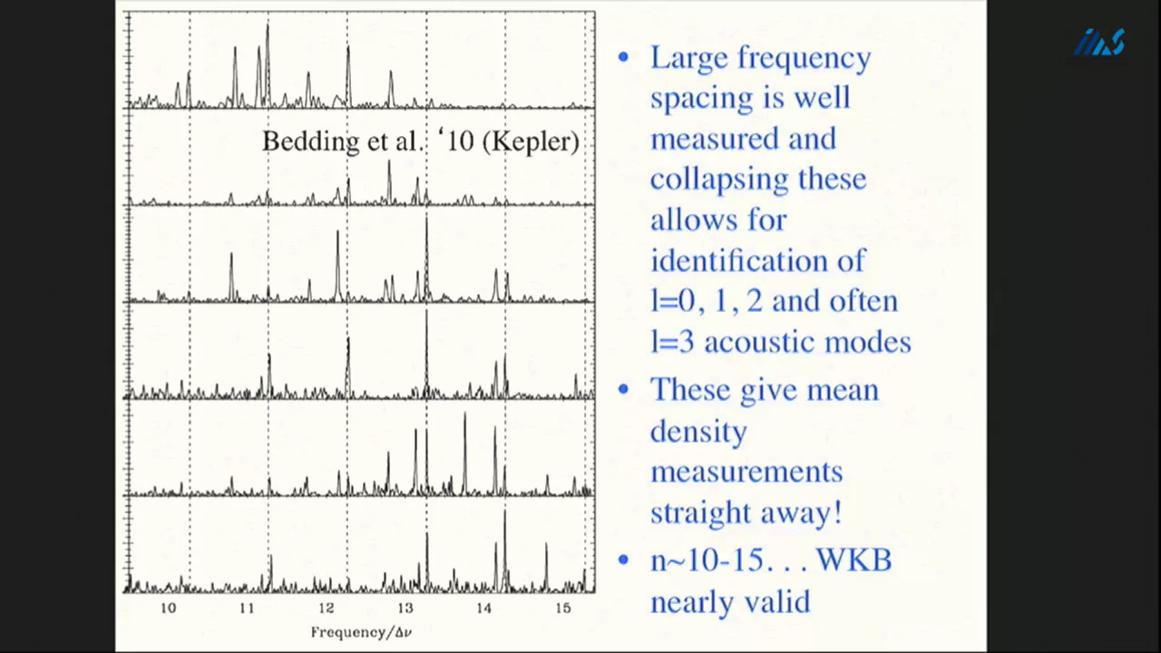
[00:00:01]morning everyone welcome to the seminar series uh today we have uh Joe on uh visitor from Hawai University he's a NASA habo fellow there right now uh originally he comes from Singapore where he did his uh Bachelor studies and then moved to Yale University I believe for a master degree and and PhD uh program and uh obviously after that moved to the University of Hawaii so he seems to uh like the United States very much uh he specializes in theoretical Astros seismology I believe with the focus on evolved stars and today he's going to talk about uh mixed modes so please Joe hi uh does it work cool uh thanks for the honor of speaking to you uh so as Tom Andrew correctly says I'll be talking to you about mostly evars um and I know that there are experts on seismology in the audience so I hope they will forgive me for spending some time providing some background and motivation for why we want to study these evolved stars in the first place okay so um I specialize in studying a particular kind of star known as a solar like oscillator right and um the reason why we study solar like oscillators uh or for that matter study seismology in general is because everything we know in astronomy is built on Stellar astrophysics and seismology is one of the very few ways perhaps the only way we have of looking directly at the inside of a star and that's how we are we better understand Stellar astrophysics right so solar likee oscillators occupy only a very narrow range of uh very narrow area of the kingdom of stars so this is a head spring Russell diagram uh showing in various patches different kinds of variable star and Sol like oscillators only occupy you know this part of the HR diagram but that's still sufficient to generate create a very rich set of phenomenology that I'll spend most of my time today discussing so what is a solar like oscillator well if you look at the sun um over sufficiently fine uh temporal resolution you will notice that it varies over timee the sun is a variable star and this this elicits some surprise every time I give an dark reach talk but is true um if you look at the sun in photometry this is what you'll see you'll see that there are uh you know inhomogeneties on the surface if you look at the sun in radial velocity you will also see in homogeneities in radial velocity superimposed on top of the rotational uh red shift and blue shift that arises from the rotation of the sun right and the these inhomogeneities uh emerge from local velocity structure arising from you know just random conviction right and you might think that this is entirely stochastic but if you were to average this over the visible dis of the sun um you would get um variations in radial velocity that are coherent and the reason for this is that these tiny stochastic variations in the in the fluid velocity field coupled to Global Acoustic oscillations sound waves that may interfere with themselves constructively to yield normal modes of oscillation so these are the pul stations that we're interested in okay so if you were to integrate the radial velocity uh well these radio velocity structures over the entire visible dis and keep track of how they evolve in time they will appear not to stay still but to vary over time if you were to look at these variations in the frequency domain by taking a fora power power Spectrum you would see coherent Peaks right so each peak in this Foria power Spectrum corresponds to a normal mode of oscillation you see that these Peaks form you know more or less evenly Spaced series of modes right so each each evenly Spaced series of Peaks uh corresponds to a family of most with the same horizontal shape which we will get back to later and the characteristic spacing between these overtones of modes in the same family we call Delta U the large frequency separation you can think about that as being proportional to well depending on the sound travel time of the Sun in the same way that the spacing between overtones of a pipe or a flute also depends on its sound travel time okay so the characteristic property of these solar like oscillators is is that you see lots of modes at any given time right and that's because of the stochastic nature of how these modes are given kinetic energy they are pumped by random motions uh owing to convection and because of this basically every mode which can have kinetic energy uh close to some characteristic convective frequency will have kinetic energy and this makes life pretty easy uh when we want to interpret Peaks that we see in the power Spectrum okay so in principle we could do similar analysis for stars other than the sun we could measure the radio velocities over time take power Spectra and see and look for either peaks in the power Spectrum or if we don't see Peaks at at least look for an overdensity of power in the power spectrum and this is a map of every Star we did this for uh from 1995 to about 2008 uh that that's not a very that's not a very large number of stars right that's because because taking radio velocities is very expensive you need to Commander a telescope to stare at one star for days at a time with a Cadence of maybe one taking a picture of a star you know maybe once every few like every couple of minutes so that's not economically feasible uh and uh it turns out that most interesting stars are not that bright so we can't even take radio velocities of them anyway so the mitigating strategy that uh scientists have turned to over the last now decades is that rather than taking radio velocities we take dis integrated photometry so we measure the variations of the brightness star and how the brightness of a star and how it changes over time right you can do something similar you can take a power the power spectrum of this brightness and if you see peaks in the power spectrum of the photometry then you can play the same game you can say these are normal modes and you can interpret the normal modes in the same way as you would those in the sun right so we've been doing this for two decades now since M um most recently we've been relying very heavily on Kepler and K2 and uh in the last well since I started my PhD a lot of focus has been on tests which is the the currently active uh photometry Mission run by NASA so so far I've been talking about solar like oscillators right and um it might also perhaps not surprise you to learn that most solarik oscillators are not sun-like Stars right so the the word solar like refers to the kind of oscillations in these Stars rather than the kind of stars that the oscillations propagate in so if I were to you know show you the power Spectra that we obtain from space for a number of stars of different surface gravities whose positions on the HR diagram you can see here you we will see some Trends as the surface gravity of the star decreases right so as the surface gravity of the star decreases or equivalently as a star gets more evolved and hits up uh hits up the the high track um as it goes off the main sequence you can see that the characteristic frequency of these pations decreases right and because of this we are able to use our measurements of this characteristic frequency and of the characteristic spacing between normal modes to make some inferences about the properties of the star so these are these properties are known to scale with the global properties of the star the mass radius temperature and so forth in in that fashion and we can invert these scaling relations to apply seismology as a tool for Stellar characterization right so from these scaling relations for the global seismic properties we can obtain estimates for say the mass and radius of a star and this can be very widely and quickly applied to a very large number of stars at once because it doesn't take a lot of effort to measure um the large separation or the characteristic exitation frequenc given the power spectrum and you can use this basically to do you know all Sky mapping of masses of stars over the entire galaxy for example um but with access to individual normal modes of oscillation you can go further like I said earlier you can use this to examine the interior structure of a star and you the the capability to do this is more restricted in the sense that that that we only have good enough quality data to do this with a significant with a significantly smaller number of stars at least least on the main sequence but um the defining property of post main sequence solar like oscillators is that the mode frequencies look very different from those you would see in the Sun or a similar mean sequence star so uh in order to better understand what I mean by this I'm going to have to rearrange this power Spectrum into a form that makes it easier to reason about the structure of these double modes right so I'm going to faceold them in the following fashion I'm going to break the pal Spectrum down into chunks equally spaced by the characteristic overtone spacing I will vertically stack the chunks so this is face folding right in inreasing order of frequency and when stacked in this fashion the power Spectrum appears to have some kind of three-dimensional structure which we will look at from above right so this three-dimensional structure is in the form of several Ridges of power right you have vertical lights and if the overtone spacing of the modes were completely constant you would see exactly vertical lines right but they're not you see deviations from verticality and that tells you things about the inside structure of the sty so each of these ridges corresponds to a different angular degree L that is to say a different horizontal shape of the modes right so this blue guy here corresponds to alal Zer these are pulsating in uh you know breathing modes and they are spherically symmetric the orange Ridge over there corresponds to dipole modes this gray one corresponds L L equal to quadruple modes and so forth right so in the main sequence star the nice thing about solar like oscillators and what allows us to do inference so easily is that when put on an aell diagram the modes look very clean they form vertical rigids so I'll show you what happens when you go off the main sequence uh as we evolve a star off the main sequence and across the head SP gra you can see additional modes coming into the picture interacting with the more or less vertical and you know doing complicated things that are very difficult to describe in words but you can see on animation that something is happening that's complicated right so what's happening here is that in these post main sequence stars there are two kinds of waves so in the main sequence stars that I just discussed there are pressure waves which are excited in the envelope and which propagate isotropically given the disturbance to the Stellar structure in these postp sequence Stars we also have gravity waves or boyy waves where the dispersion relation which I'll come back to in a minute is different what that means is that they respond differently to perturbations to the Stellar structure so these are the same kinds of ways you would see perhaps you know in on the surface of a pond where if you punch the pond downwards the waves don't radiate downwards they radiate horizontally outwards from where you punched it right so the physical properties of these waves are different and because of that uh the frequency ion values are also different so what happens over the course of Stellar Evolution what and what that this is what makes the evolution on the earlier plot so complicated is that over the course of Stell Evolution the P modes which are shown at large amplitude here decrease in frequency and the g modes increase in frequency like so right Additionally the PNG modes don't C don't propagate independently they talk to each other uh in uh in a fashion that I'll describe more quantitatively soon right so this coup between the p and g mode cavities means that over the course of stellic evolution a g mode and a p mode which come into resonance will exchange places right so this g mode becomes a p mode as a star evolves and vice versa this formerly P mode becomes g mode as a star evolves so if I were to unwrap this animation uh to put time on the horizontal axis what happens is that on this diagram if we were to make the P modes know move on horizontal lines the G modes increase in frequency but the actual normal modes the ones we actually see uh evolve on these blue curves they kind of interweave between the two families of possible modes right and they avoid the intersections of the two families of cures and this is why we call them avoided Crossings so these avoided Crossings are the reason why mixed modes are tremendously tough or legendarily tough to work with and they are the focus of my talk today more or less okay so where do these avoided Crossings come from and why do they make life so difficult uh in order to understand this I'm going to have to walk you through some Physics which I apologize for but you guys probably you know like physics anyway so okay so um in your undergrad physics courses you might have SE something like this this is called a wave equation right and it relates the temporal evolution of a wave to its spatial structure right so in a simple medium which is you know homogeneous isotropic you can pretend that the speed of sound is constant everywhere and doesn't depend on position or time right and in that case the wave equation looks like this so since everything here is constant more or less except for the wave itself which is the function f we can take for your transforms on both sides of the equation and we realize that uh you can just divide out the for transform with the wave itself and this gives us a relationship between the frequency of a wave and its wave number which is one basically one over the wavelength of the wave right and this is basically if you've written an equation of the form you know V is equals to F frequency times wavelength that's that's it right and this this is a very good description of waves like sound waves like the kind I'm making and which you're hearing um if you have a more complicated kind of medium right then you could in addition to the Sound Speed also have an additional constraint that for example the refractive index of the medium may be changing as a function of position right so we can encode that behavior in terms of what we call an acoustic cutter frequency which is position dependent because the wave has to turn around somewhere right and in that case we can't directly take the spatial forer transform of the wave although we can still do it in time but what we can do is we can pretend that we have some function uh of position uh that in in the limit of the wavelength being infinitely small acts like one over the wavelength right we call this a propagation discriminant and uh the the way we interpret this this discriminant is that the wave is allowed to propagate like normal where it is greater than zero and decays exponentially where it is less than zero right so uh for illustration I've shown a scenario where the acoustic cut frequency is shown at the solid line in this blue shaded region the wave is allow is allowed to propagate and in the unshaded region it is not allowed to propagate right so the way behaves like that you have you know oscillatory behavior in the permitted region and exponential behavior in the Forbidden region okay so the dispersion relation in an actual star is more complicated than that so there's two two kinds of oscillatory regions and everything else is forbidden right so in particular in a red giant whose interior structure I'm showing the two different propagation regions exist uh are those near the surface shown in Orange where P modes are allowed to propagate and those in the interior shown in blue where G modes are allowed to propagate right so this is the kind of you know Brute Force numerical approach that or or know quasi and analytical approach that we've been applying so far and it's helpful in terms of classifying where the waves are exhibiting what kind of behavior but it's less helpful in terms of actually doing calculations which we've still been using Brute Force methods for so I'm going to walk you through an alternative formulation uh with perhaps a different way of conceptualizing the separation between the g- like Behavior and the p- like behavior of these modes if you've taken a chemistry class this might seem somewhat similar familiar right so I'm going to walk you through first a construction that's commonly used in physical chemistry uh called the method of molecular orbitals and the method goes like this let's say that you fully understand the igen system of a particular atom say the hydrogen atom right and now you want to make a molecule out of two hydrogen atoms now if the two atoms were at infinite separation then the ion states of the combin B system are just two copies of the hydrogen atom right that's pretty easy but if you were to bring the two atoms together to form a molecule what you can do is you can treat the hamiltonian with a combined system as for example the hamiltonian of atom number one plus a small perturbation from atom number two or vice versa right and as you do this what happens to the igen states as you reduce the interatomic separation is that they become combinations of the of the atomic orbitals of both atoms right so the ground state will be the ground states of both atoms interfering constructively the first excited state will be the ground state of both atoms interfering constructively right and the difference in energy between the two can be written as some overlap integral between the two ground state wave functions or the two atoms right so there is an voided Crossing hidden here as well in the sense that if rather than considering a diatomic hydrogen atom you consider a diatomic hydrogen like atom in the sense that you permit the charges of the two atoms to differ in that case the two the first and sorry the ground and first side states of the molecular system exhibit an avoided Crossing in terms of the charge ratio of the two atoms right and you can see that qualitatively when they are far from resonance they behave just they they are you know very similar to the ground States of the atoms considered separately and when they are close to Resonance then they are very strongly mixed right when they are far from resonance as well they can also see that the difference in the energy I values appears to be a root of some polinomial in this case of degree too so this is very suggestive of uh being the igen values of some Matrix and actually that is exactly the case in the limit of many uh Atomic orbitals interacting with each other to form molecular orbitals what you would do is that you would Express each molecular orbital as a linear combination of atomic orbitals with the coefficients of this linear combination being given by the igen vectors of some overlap Matrix and with the igen value specifying the energy levels of each molecular orbital so the situation in seismology is actually surprisingly uh entirely analogous right you have your you you have waves normal modes generated by sub wave equation which can be expressed in operator form and you can express the operator generating these mix modes as perhaps a g mode wave operator with a small perturbation from the from from the P mode cavity or conversely as a p mode wave operator with a small perturbation from the g mode cavity and if you want to express your mix modes as a some linear combination of your p and g modes then you just use exactly the same Matrix Machinery right you compute the same kinds of overlap integral of the full wave operator with respect to the P PNG G modes you put them in this big Matrix you solve for the igen values and you've gotten your mix mode uh and you get your mix mode igon values with the igon vectors telling you what the combinations of PNG modes ought to be for each mix mode okay so with this technology in hand we are now able to uh better interpret the p and g components of a set of mix modes presented to us observationally right so for example one thing you can do is given a set of GES you can put them similarly on a shell diagram and by doing some clever coate transformation you can get the mix modes to give you what the PG modes ought to be and you can interpret these prg modes in terms of rotation I'm going to skip this part or in terms of magnetic fields which some members of the audience Have Been instrumental in this covering um and I'm going to point out some student work also uh to do with interpreting these magnetic fields so Nicholas royy has been working on you know nonlinear peration Theory um for interpreting uh strong magnetic fields in combination with rotation in G of faders and Emily hat who is at the University of Birmingham has been working on cataloging extensively the strengths of magnetic fields in many many red giants all at once using automated techniques but I'm not here to talk to you about G modes uh today I'm going to talk to you about the P mode components of these mix modes which has so far largely been neglected so returning to our observational diagram we have for a main sequence solar like oscillator a set of vertical ridges on it a shell diagram right and we can think about not just the large frequency separation which is the overtone spacing required to obtain this diagram by face folding but also the separation between different ridges on this diagram so of particular historical interest to the people studying sunlight Stars has been What's called the small frequency separation which is the separation between this Ridge and this Ridge right so that's the separation between the radial modes L equals 0 and the the quadruple modes L equal 2 so that's labeled on this diagram as Delta new 02 all right so the reason why this historically been interesting is because if you do some math uh you will eventually find that for a main sequence Sun like Star this quantity depends basically only on the interior structure of the star so it doesn't depend on the near surface layers of the star additionally uh its precise dependence on the interior structure of the star uh is on the Sound Speed gradient near the center of the star so this the this expression is saying that the small frequency separation is a weighted average of the Sound Speed gradient or the star with the with weighting increasingly heavy towards the center of the star now as a star evolves of the main on the main sequence the chemical composition of the nearest Center changes over time right and this causes the chemical composition and therefore the Sound Speed to change in a in a position dependent fashion over at the ca of it main sequence burning and as such uh the small separation can therefore be used to accurately measure Stellar ages for main sequence stars and so for this reason it has been used uh as a direct asmic probe of the Stellar age so let me show you what I mean if you were to plot the small Separation on the vertical axis against the large Separation on the horizontal axis for a set of computational models of Stellar structure uh what you will obtain is for uh for a star a constant Mass uh the star evolves along these a star will evolve along colored curves like these right if you were to plot lines of constant age on this diagram these are isocon uh these will follow these uh the isoc cones follow these dashed lines intersecting The evolutionary TRS right so what um so I've been talking mostly about the small separation Delta new 02 but if you were to divide the small separation by the large separation you get What's called the separation ratio so that's r02 in some of my slides if you were able to measure r02 and the large separation and put it on this diagram you will see that basically by placing a point on this diagram you you will be able to just read off a stellar age from this diagram right so that's why people have been so interested in you know making measurements of the small separation or the separation ratio for main sequence stars but you might have already noticed something strange about these diagrams which is this you know messy grossness here so any guess us as to why that is so there is a clue in one of the animations I showed out there which I'll show again okay so again I show this animation and I want you to pay attention to the small separation as the star evolves of the main sequence so think about this from uh perhaps a computational perspective how would you compute a small separation given this rapid Evolution right you won't so what what happens is that if you were to compute the full set of mix modes here and attempt to to measure a small separation from these mix modes you will get a lot of numerical noise simply from the avoided Crossings happening as the G and P modes come into and off resonance but that's a problem that we've just solved we are now able to compute po modes from Cellar structure and as such we are able to compute the smooth evolution of the small separation or equivalent separation ratio for sub and red giant Stellar models and so if you were to do that calculation uh that's what this is what you would get it's a smooth curve right over the course of Stell Evolution Stell the star evolves from Zer H main sequence here on the right and as the star goes off the main sequence and up the red giant Branch it heads to the left and the small separation decreases over time like so so that's a first um but what happens if you were to compute that integral estimator we saw earlier the integral of the sounds gradient as a function of over the Stellar radius if you were to compute the estimator for the small separation this is what you get right so um the the small separation is supposed to be strictly less than the large separation so some something has clearly gone wrong uh here and correspondingly this means that we cannot interpret the small separations that we observe in the field as being related to this integral in any fashion okay so what's gone wrong um to understand what H what happened uh we first have to attempt to understand where this expression came from so I will try to do this without going into to the weeds too much um what I will do is I will describe the normal modes uh you know in terms of their radial displacement so over the course of one oscillation cycle at each point in the star the fluid is displaced in the radial Direction by a little bit in a periodic fashion right uh I will describe this as a function not of the physical radial coordinate but in terms of the acoustic radio coordinate the sound travel time from the center and I will scale the I functions in a clever way so as to make the pulsations look more or less sinusoidal as a function of the acoustic radial coordinate okay so what happens is that when you perform this coordinate transformation and this scaling you can approximate the the normal modes as being more or less cidal up to an overall phase upset right so for radial modes for example we need some phase offset that I've shown in this slider and let say for Lal 2 we might need a different phase offset in order to get agreement with the actual normal modes we compute numerically so it turns out that the small separation or more accurately the small separation ratio uh can be expressed compactly as the difference between the phase offsets for the quadruple modes versus for the radial modes okay so what went wrong is that when when we derive the relation between the small separation and the internal structure of the star uh we are actually making some small angle approximation in the sense that the integral the integral expression we have tells us not the phase offset per se but rather the tangent of the phas offset right and when we relate the small separation to the Sound Speed gradient we are in effect making a small angle approximation so let's see how valid this approximation is I am plotting on these figures um the the quantity Theta entering into our expression for the small separation for sorry for the inner face offset right and this I am showing for a main sequence star so in order for the small angle approximation to work we need these curves to go below one um at some point in the S structure and this assumption is well satisfied for the main sequence model shown here for a red giant however uh this quantity never goes below you know 10ish right and as a consequence of this the small angle approximation that we are requiring for our integral estimate for the for the small separation breaks horribly for sub Giants and red giants and and the remediation for this is fairly simple we just don't make a small angle approximation and compute the full you know arc tangent or whatever and we get now a slightly more complicated expression for the small separation ratio so in the limit as these quantities go to zero we recover the existing expression that we have in hand for the small separation ratio but in the opposite limit which is what we encounter in red giants um it turns out that a small separation doesn't actually depend on the internal structure or at least shouldn't depend on the internal structure of the star it goes instead as some ratio of the large separation and the characteristic exitation frequency uh um and that's a bit hard to believe right so let's do some numerical tests so here I have plotted the small separation ratio of a series of Stellar models the same ones that I've shown in the earlier figure where I showed the small separation itself and here I show um the values of our modified estimator with the limiting values in the in the limit of it not depending on Stell structure shown with a dash line so there is an offset between the values return by our approximation and the values that we compute numerically from the solar structure so there aside from the constant offset between the two which we can explain with higher order effects there's also a bump here that we cannot explain with higher order effects right um and we might wonder whether this might be interesting in terms of our ability to peer into the inside structure of the star so recalling what I said earlier about the small separation ratio depending on the difference between the radial mode and the quadruple mode interface offset we can decompose the SE the difference between the two in the contributions from the radial modes and from the quadruple modes and where we see the bump in the in the separation ratio we see a bump in the radial modes phas offset but not in the quadr mode quadral mode phase offset and that indicates that if the bump depends not anything any property of the cellar structure that feature in the cellar structure has to lie quite deep into the star right and one feature that does lie quite deep in the star in these rather evolved stars is the boundary of the convection zone so here I show basically how the bound where how the position of the boundary of the Conant Zone evolves over time right and as as it does so I also show on the right panel where we are on the christard diagram the the on the figure with the separation ratio on the vertical axis and the large Separation on the horizontal axis and what we can see is that uh on this side I'm showing basically the amplitude of the wave function and the at frequencies close to newx um and what we can see is that where the bump happens on the right panel corresponds to where the convective boundary passes over the innermost maximum of the wave function close to newx and we can interpret this uh SE as we can unwrap the animation like so right um the colors of this figure represent where the waves have highest amplitude right and where the waves have highest amplitude coincides with where the convective boundary of these evolved stars is at frequencies that always coincide also so with where we are seeing the bump in the small separation ratio so we can conclude from this that if we see the bump in the small separation ratio that means that the convective envelope currently is sitting at the innermost maximum of the P modes that we have access to in the star so that's it that that that's the interpretation um and this is a lot of theory work um but I'm quite excited to also announce that this has recently been observationally verified so uh Claudia rise who is uh a finishing PhD student at the University of New South Wales um did a Ensemble of measurements of the small separations for red giants in the open cluster m67 she put them on this diagram she calculated a Stell evolutionary track with a certain amount of overshoot and the small separation measurements line up exactly on the track and and that pins down basically the behavior of the convective boundary um as a function of time now precisely what Behavior do I mean this all of this discussion concerns the position of the convective boundary and how it moves in as as a star evolves right but in a real star um the position of the convective boundary is not quite the same as we would expect in our approximation for stars satisfying spherical geometry and that's because convection is a highly uh non one-dimensional process right in general convection happens in 3D and as such defining the position of the convective boundary is always a bit difficult in particular because convective plumes have some velocity they can always overshoot the boundary of where convection is stable versus where it is not so phenomenology Al what we would see in a 3D hydrodynamical simulation like this one is that you have mixing of the star extending beyond the region of convective stability this is called convective overshooting right and it is the position of this mixing rather than the the position of where the convection where convective flows are stable that actually defines where the convection Zone ends as seen by seismology so to put things differently our our ability to probe the position of the convective boundary using seismology effectively permits us to constrain how much convective overshooting is happening in these m in these red giants right so if you were to examine how the small separation Ratio or equivalently the differences between the interface offsets depends on the amount of convective overshooting which is shown by different colors you see that there is some sensitivity um I unfortunately didn't put observational error bars on this um but the the the separation between the curves is comparable to or larger than the the observational uncertainties that you would get right so this is the basis of our next search for convective overshoot which we just got funding for uh from NASA okay so to wrap up um red giants exhibit mix modes which behave like G modes on the inside of the star and behave like P modes on the outside of the star these mix modes may be described as acoustic molecular orbitals in a publication that I wrote you know a couple years ago using this separation between the p and the g modes we can extract information from the P modes and we can remediate a broken small angle approximation in our existing theory of P modes this remediation of the small angular approximation leads to new new theoretical predictions for how the small separation ratio depends on convective overshooting which has recently been observationally validated so yeah that's it right I've talked about understanding M modes as an object of Interest per se that's the fun part and I've talked about using this new understanding to constrain the physics of convective overshooting that's the profit so that's my talk thanks for your attention thanks Joe for an interesting and uh very clear talk uh time for questions we have about 15 minutes don't be shy thank you for the nice talk I'm one of the non asro seismologists so I'm more interested in the The Mixing stuff um because I'm doing Evolution so you have shown this overshooting parameters how is overshooting in this models you have shown implemented is it step or exponential overshooting and ah these are models generated with exponential over shooting right so are you familiar with Mesa yes so um the sorry yeah the parameter fov here is the fov parameter for mesa's implementation of exponential overshooting yeah um I will also say that in our observational paper we compared the experim the you know observational values of the small separation ratio against evolutionary tracks generated with no overshooting and with twice the prescribed amount of overshooting right you can see a difference here and the lever arm is provided by this particular feature in the small separation diagram thanks more questions uh hi yeah and thanks for the Fantastic talk I was just wondering um so in terms of the quality of data needed to do this kind of analysis like you've shown an example here was this like an unusually high quality data set for this star or are there many stars that have this good data that you compare with which star do you mean say this one the one you've got on the so this is an open cluster which means that we have light curse for several Stars um I I think the data here is not of unusually good or bad quality this is more or less standard short Cadence uh K2 data so there are more instrumental systematics than the nominal cap Mission but it's also not as nice as a nominal cap Mission but it's also not as bad as for example the instrumental systematics that we associate with tests where you have like know large separations between individual windows so I think the important thing that we require for analysis of this kind is data sets of unbroken length um which is difficult but not that difficult to come by okay thanks more questions um in the diagram where you showed the evolution of the um separation ratios somewhere on your like 50 something on the slides uh where the where you had the tracks exactly like one of these okay um I was noting that the sun is not on the one Soliz track can you comment on this I know it's not your work but uh yeah I didn't make this so um one issue with putting things on this diagram is that um the position of things in the horizontal Direction depends on systematic errors that we make in modeling the Stars right this is called the the surface ter or near surface effects and this can affect the value of the large separation we compute from a star from a stellar model with exactly the same Stellar structure as something we see in the field so for example if you were to compute the large separation for a solar model you would get something like you know 140 microz uh even if it's even if its internal structure is exactly identical to that the Sun but the sun gives us a large separation of 135 microz and so it's the horizontal position that changes but for the small separation ratio diagram you can see that the horizontal position doesn't really change the estimate of the AG you have and so that's not that big a deal thanks for the great talk um I was wondering you uh when you showed the result for the cluster um each point was an individual star uh but I always think like if you have multiple modes in a star they will slide well where they prop differ slightly so could you learn something about where the uh well how the the the overshooting region looks just by looking at all the different individual separations in principle you could um we didn't do that for the N for the observational work because the data were not of sufficiently high quality for us to do individual mod fiting so what we did for Claudia's paper is a bit uh different I don't have a slide for this unfortunately but you can kind of visualize how it works from the shell diagram I think so so the the the technique CL use is called the collaps the shell technique where you f you first begin with a candidate large separation which gives you an a shell diagram like this but it looks very noisy because you know that is not the high quality then you you project in the vertical direction and you just see know two peaks here and one Peak there right and the the separation between the two peaks here can then be used as as as an estimate for the small separation but you are correct if you were able to do individual frequency measurements then you would you would be able to get still more detailed information about the convective of a shoot follow thanks for the very nice class Joel replacing my whole course this semester thanks a lot you did it in less than one hour um um following on Vincent's question can you actually do an inversion for the I mean cor overshoot is really just a a term to replace a whole bunch of opportunities that may occur and may intervene between rotation magnetism and waves even well you could you could do a in principle if you had high quality enough data you could do an inversion for the position of the C of the convective envelope boundary um the reason why we haven't done it is kind of described in this figure so um I show with the blue points um the entire cap sample of oscillating Stars right and um the region of Interest where we have sensitivity to the convective envelope boundary that's shown in Gray um you will note that it kind of Lies mostly in the gap between the long and short CAD of cap so this is why we haven't been able to do it with capital data because we just don't have we just happen not to have any stars lying here as a result of the observational window function but in principle um you know test is going to soon have four years of data so perhaps we might find a star lying here in test we've identified some already shown in Orange and so that those will be our first targets to look at stand for more questions hi Joel thanks for this nice talk um I was wondering so you showed for your cluster as well but you only have one small frequency separation but I guess you could use is it possible to use both of them like you have two for the P modes right for the L equal to Z one two and three ah yeah so if you go back to your iSell diagram you actually I guess maybe the difficulty is that you don't really see the the other rich like the gray one the dark gray one here sometimes yeah the elal 3 small separation is really hard to pull out U because this is just from geometrical effects right because as you integrate over the whole this then the power the visibility of higher and higher degrees just gets washed out by geometrical integration yeah so as far as I'm aware we have L equals 3 mode measurements for some stars from Kepler but this is very hard from photometry so if we wanted to get Al equal 3 modes in principle we should be you know trying using groundbased radio velocities because the projection effects just work in our favor there but groundbased radio velocities are expensive and really impractical for getting you know a yearlong baseline of the kind you would need for inversions okay cool I was wondering like what what what can you do extra if you have this available then so what what can you do extra if you have the the L equal three yeah if you have the L equal 3 mode in principle you get more more resolution and the radial direction for structural inversions because different families of L have different inner turning points right so for example if all you had were just the overall phase of the modes you could still do a very Co kind of inversions by taking you know the difference between the L = 1 and L equal 2 in in in turning points and that that's one resolution element right so with L equal 3 modes very roughly speaking you get one more resolution element further out from the center okay okay thanks still have some time okay uh more more questions of what mixing so you have shown the that you nicely can determine like the O extent of overshooting and I wonder um how sensitive are your results to other mixing parameters for example if you use mixing uh as for MLT standard MLT um if you change your Alpha MLT value like your maxing length it would change like the structure of your star and also should impact like your um derived overshooting that is true so ultimately this will impact the inter interpretation of our results in terms of overshooting right so at the core what we are truly sensitive to is the position of the convective boundary um so in principle one could eliminate dependences on choice of alpha MLT by doing something like an entropy calibrated uh entropy calibrated mixing things and um know there are alternative formulations that extend or don't do away with mix and length Theory altogether um the the important thing however is that having an observational handle on where the convective boundary is permits us to validate these theories in general not necessarily in the form of overshoot thanks Plato will allow you to do that launch is December 2026 yeah s uh thanks so it was a very like Clear Talk for so thank you for uh dive into this uh field so um my question is regarding radial velocities so for the solar Stars I think you showed a sub meter per second diagram in the beginning introduction uh for let's say F stars or do you expect larger uh oscill like larger signals in the radial velocity space uh and like what is the like maximum you would like in terms of precision uh go for to characterize F Stars okay uh so that's two questions yes uh so the first the first question is um what what kind of rate of velocity Precision we would expect yeah so sorry what kind of rate of velocity amplitude we would expect for an fstar right and that's of all like half a meter per second uh second question was whether we could use it to characterize F STS the answer is we thought so but the answer is probably not and the reason for this is not what you might think so um in these power Spectra you will see that the individual modes are really well resolved right so you can see narrow peaks in the T Spectrum in the F in an F star the lifetimes of the modes are really short so they they stay they stay coherent for a really short amount of time and what that means is that the modes are really fat in the power Spectrum right so if you were to make a similar a shell diagram for an fstar the modes are so fat that you can't tell the L ital zero and two modes apart right and so that that limits the amount of structural information you can get from that ST which is why we we've generally not so far been too interested in small okay thank you still some time not much but maybe for one two questions in the meantime Joe maybe if you could go back to the oh forward to slide 77 um so what I've have noticed there on the run right hand side uh plot yes that there is some noise and that noise seems to be increasing as the overshoot parameter decreases which is suggestive of some numerical issues in the models yes so what what's wrong with our numerics and if there is something fundamentally wrong how can we actually use these models as a tool uh okay so this this is a specific issue with the version Mesa I used to make these diagrams um so this ultimately is to do with how we Define the position of the convective boundary right so when there is no overshooting you would Define the position of the convective boundary as basically where the Str Criterion changes sign right um the problem is that um by default um Mesa doesn't remesh the neighborhood of the convective boundary more finely in order to to more accurately give you this so because of this the if you were to keep track of the position of the classical boundary as it evolves there is there's going to be some numerical Jitter right and as as a consequence of this numerical Jitter you also get Jitter in the mode frequencies um so this is actually fixable uh it's just I didn't fix it for this figure sorry about that so it's a it's a resolution effect that you can solve with like adaptive meshing or something okay um so that there used to be and there now is again uh this a long story uh an option in Mesa called convective boundary weight right and that tells you how many more mesh points you need to add to the model near the convective boundary in order to smoothly resolve it so this was removed in version 12778 and only very recently had it back again yeah okay thanks all right um maybe one more very last question if you will want to no then let uh thank Joe again for his wonderful talk thank you for having me so I believe Joe is still around today so don't hesitate to approach him and talk if you want to need to yeah and tomorrow as well thanks