









![The Dark Energy Mystery [4K]](https://i.ytimg.com/vi_webp/cQyoYzHxdvo/maxresdefault.webp)








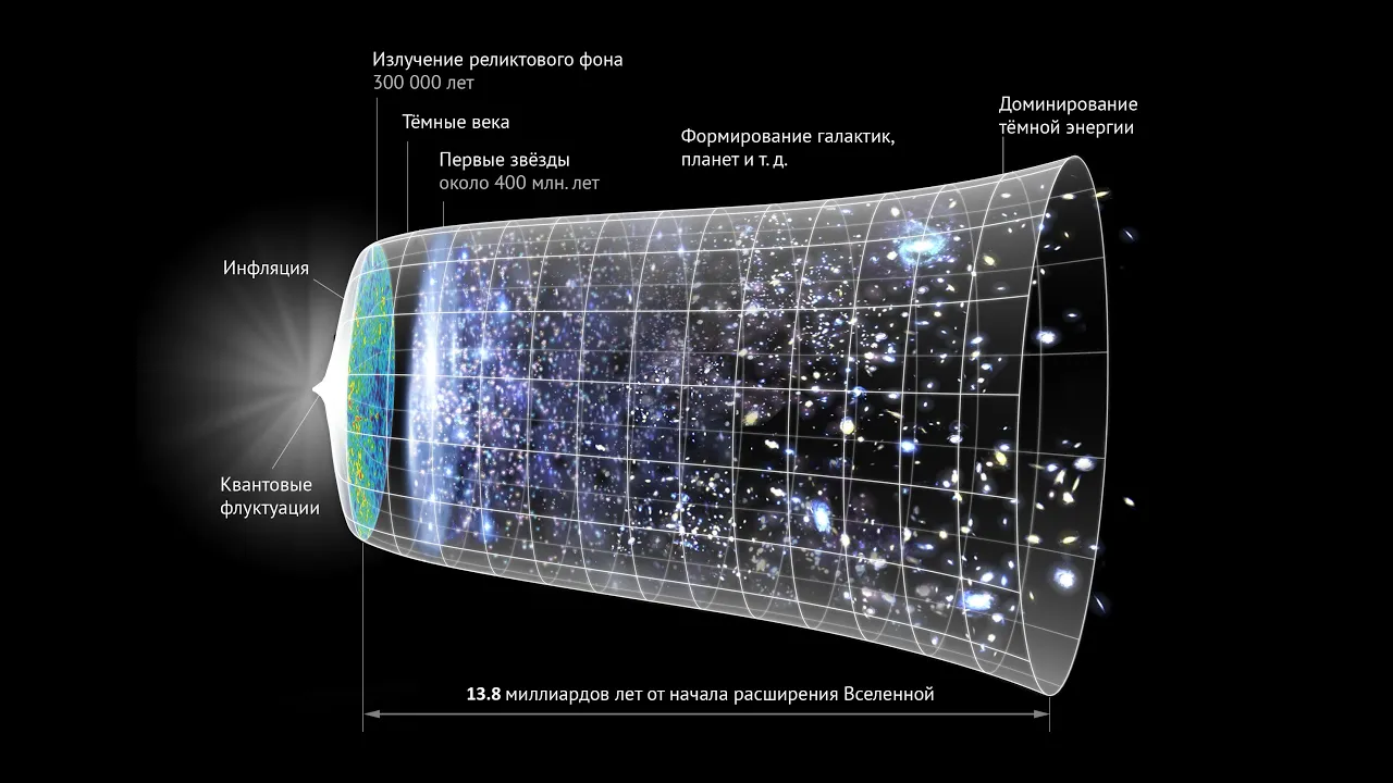
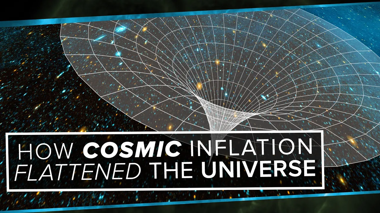





This lecture introduces the foundational framework of cosmology using the Friedman-Robertson-Walker (FRW) metric, which describes a homogeneous and isotropic universe through the scale factor a(t) and curvature parameter K. The cosmological principle states that the universe is uniform on large scales, enabling simplified mathematical modeling. Key concepts include the Hubble parameter H = ȧ/a, the Friedman equation relating expansion rate to energy density, and the continuity equation governing how energy densities evolve with scale factor. Different cosmic eras emerge based on dominant energy components: radiation dominates early (w=1/3), matter dominates later (w=0), and dark energy (w≈-1) currently dominates, causing accelerated expansion. The particle horizon problem—where causally disconnected regions appear to have the same temperature in the CMB—motivates inflationary theory as a solution.
Introduction to Cosmology: Lecture 1 by Laura Covi | GR Basis & FRW Metric
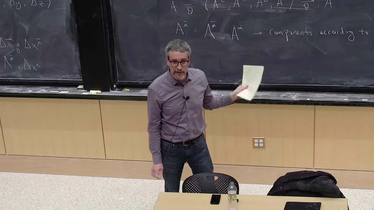
Added:so very happy to be here and to see that you're so numerous you have I didn't expect it to have such a full room but nevertheless let's I decided to start a little bit from the basic since the title of the lecture I've been given is introduction to cosmology so I hope it will be not too much repetition today for people who have already had a course in gr on cosmology but just to setting the stage today we will be practically the basic stuff of cosmology then tomorrow we will show the plan of the lectures is the following so we have so today we will have the introduction with a bit of general relativity and cosmology tomorrow we will go on with again the part of the if you want more classic side of cosmology which is the practical inflation and the cosmological perturbation and then on the third lecture we will go to the thermal universe and there we will discuss a bit Big Bang nucleosynthesis and we will discuss also Dark Matter what is the start and then in the last lecture on Thursday we will continue on the thermal universe again bit on other candidates of dark matter and if we get there some elements of biogenesis but I think you have also lectures on it now in last week if I remember correctly so I will not really go to the detail I will try just to get there so that you can get a connection later on okay so this one is the plant of course it's a bit optimistic say especially because it's done on the blackboard usually the rhythm of the blackboard is a bit slower so I'm not sure I will be able to cover all in the case also it's probably not important that I cover all is more important you understand what I cover and so you are welcome to ask question and in any moment and we can stop any moment to check if you didn't really understand the things so that we have at least a good foundation for the rest of the school okay so introduction to GR the first element we have a little bit to cover is the general relativity so of course these should be clear that this was the beginning of cosmology before Einstein before they were writing down general activity nobody really knew how to describe the evolution of the universe okay the idea before was that the space was actually static it was kind of absolute space and time was a variable which was completely independent and it was just a kind of sequential quantity which was more or less taking care of the evolution of the system it was only with Einstein first with the special relativity where people really realized that space and time are actually together and indeed the time is not the same for all observer and you have to do as usual well the transformation were of course known also before to change the coordinate system Hey and then later what he also realized was that the curvature and they the geometry of space-time is also a dynamical variable in that sense and this led today to general relativity but one important principle we also have in this respect in cosmology and which also was introduced by Einstein was the cosmological principle and not not only him actually not because no logical principle is also needed ingredient because without these it would be too complicated practically to describe the universe and what does the cosmological principle say the cosmological principle states that the universe is homogeneous and isotropic on large scales well I hope you know all homogeneous and isotropic homogeneous of course means that every point is more or less the same as every other and isotropic that in every direction you look you see the same universe and of course the other important thing is on large scale what does it mean on large scale well it should be clear that in this room the universe is not homogeneous isotropic in the solar system the universe is not homogeneous isotropic because you have a planet or you have war void then you have the Sun etc you need to go at a sufficiently large scale and the sufficiently large scale if you can want to have something in mind is more or less the scale of the horizon now or the scale of this sizes that you can observe on the CMB for example the CMB looks it's practically one of the largest scale we can observe and then of course also you have all the observations that you comes from a large scale structure which we will discuss briefly later on when we look at structure formation and in that case as well you see that if you look for example at the density contrast this is usually the quantity which is of interest is the density at the place X minus the average density divided the average density and this quantity is usually nowadays of order one for example on a solar system in the average everywhere where there is a structure already formed but if you go to large scale this quantity becomes quantity smaller than one so you have as I said if you go two scales which are on the order of thousand mega parsec or so you start to see that this quantity Delta is actually a small quantity of the order of 10 to the minus 3 and in the CMB for example this is also corresponding to the temperature fluctuation we choose of the order 10 to the minus 4 10 to the minus 5 okay so and this is exactly the reason why we can take the first order approximation isotropic and homogeneous universe and then on top of it and this is something we will see tomorrow if I am NOT able to introduce it today we can do the perturbations so we will use the fact that Delta is small - right for example something like omo genius universe plus fluctuations okay so so if you want background at yeah at leading order has Delta equal to zero okay and this is what I will discuss now so how can we discuss isotropic and homogeneous universe in order to describe as universe we did as usual in grr metric so this is the famous la Mettrie feed one yeah Robinson Walker and this is exactly the metric which satisfy exactly the homogeneity and isotropy and it is practically the simplest metric you can write down for a kind of homogeneous manifold with with a spherical symmetry so you have impre-- in the first part is the time which is the usual dt square so this is the same as in the Miccosukee metric but then you have a scale factor which depend only on time and then you have the three dimensional metric which generically it can be flat or curved and the generically the expression can be written in this form with a radial coordinate with a factor which depends on on a key parameter and then you have the usual spherical angular part with an R square so the Omega is as usual in three dimension is the the theta square plus sine squared theta d square Phi okay so you see that immediately that here you have a really very simple expression so you have only one dynamical variable which is a and we have one parameter which is K which I can probably write also in a different color and the rest is practically just the usual coordinate like in the Minkowski case notice of course I take the signature 1 minus minus 1 minus 1 so as usual so you can compare it to the makovski metric and the Minkowski you have a d s square is equal DT square - yeah well you could have again TR square plus R Square D Omega if you have statical coordinates what I actually don't need I think the Omega square it's usually just the Omega ok so what does it mean for the metric of course you know that I can define of course a tensor metric tensor G mu nu which multiplied for elementary a distance DX mu DX nu and therefore if you look at the metric above you see immediately of course in this case it would be just 1 minus 1 minus 1 minus 1 in this case instead the metric is again diagonal and you have again a 1 and but here of course you get a me minus a square T 1 minus K R square and on these sides you get also a main minus a square T R square sorry I forgot the R square of course and minus a square T R square sin square theta sorry in the second column sorry there is no work oh yes you're right here there is no R square yeah okay so you see immediately the advantage we have a generic alia metric we will see it also later on it's a symmetric 4x4 tensor symmetric 4x4 tens or Herricks exactly ten independent quantities so you see it immediately you have four in the diagonal three in the next two and one if you sum up the number from one to four you get exactly ten so usually if you would just write down the most generic metric you would have ten degrees of freedom for the Friedman robertson-walker metric we have only one degrees of freedom which is the scale factor a square and all the rest is practically fixed by the geometry so this is the big advantage of this metric now we have to get a little bit what is the physical meaning of this parameter K to get what is the physical meaning okay we have just to compute what is the curvature in three dimensions so to do that we just need to compute today let me turn okay so let's say then what is the meaning of K as I said I can compute the three-dimensional curvature which is nothing else as the Ricci scalar in three dimension I write it like this and if I do that I obtain something of this form yeah okay r-squared no sorry that's wrong too many factors it's a square - yeah so you see immediately that K square determines the curvature in the sense that K of course the sign of K can be positive or negative if it is positive you have a positive curvature negative you have a negative culture k equal to zero will be automatically zero converging yes [Music] three R is because it's the three dimensional curvature the three if you want a Ricci scalar in three dimension we will later on have the Ricci scalar in four dimension which will have other contributions so this will not be actually connected to the three dimensional curvature but to the four dimensional curvature now in here observe already also yes and when you have here you know so observer this depends on the scale factor a so you see immediately also that how exactly the curvature is depends on a square and the real value of K actually can be rescanned into rescaling the scale factor so what is important is only if K is positive negative or zero that is why usually people use K to define it only at their +1 -1 either +1 0 or minus 1 and the +1 is a force the closed universe positive curvature so you to think about something you can think about the sphere k equal to zero is the flat universe and k equal to minus one is the open universe or hyperbolic universes so in that case the curvature is negative it means in one direction you have positive curvature in other direction you have negative curvature and if you want usually the way to to cope with these different spaces is actually to rewrite the radius here coordinate in a different way you can redefine a KY variable which is nothing else's the R square 1 minus K R squared and solve this equation and now you see immediately that kyuf Air has three different solutions you can have an re an arc seen solution of R for k equal to 1 you can have a justice solution R where K is equal to 0 and if you are in this a case of k equal to minus 1 you get the arc sin hyperbolic goose and in this way you are practically able if you go to the variable Chi instead of the variable are you can treat all the three different species in the same way just using D Chi square instead of r and you substitute the solution depending on the value of K now in the future I will actually concentrate on the k equal to 0 case and this is not by chance is because this is what seems to be what we measure okay if we measure now the three-dimensional curvature this is practically very near to 0 of course as you see immediately here this doesn't mean that it is exactly 0 it could also mean it indeed it is also so that the universe is very large so a square is large and this means this would actually reduce the curvature so we we do not really know it the universe is exactly flat but it looks very much near to flat and therefore I will concentrate later on to the solution with k equal to 0 ok so I have down now just another important redefinition to introduce because we see immediately this metric actually doesn't look very different from the Minkowski metric we see that the part here if we would could be able to take out on a square from everything then it would look like more or less like Airy scaling of the Minkowski metric and indeed this is exactly what you can do if you redefine the time you read it fine in to be the conformal time which is defined with an additional factor of a square so this is usually useful in cosmology to define the conformal time the conformal time is I will use eta is a of ETA D ETA ok so I really that I have an additional factor of the scale factor and that it should be clearer than therefore then I have the simple metric where if the a square comes out in front of it [Music] and no air square here okay so this part is nothing else as the Minkowski metric for the conformal time though okay and this scale factor is just a conformal factor because you can rescale it conformal transformation of the metric huge or a scaling transformation of all the coordinates that is exactly equivalent by multiplying by the scale factor and this way of writing the metric has of course the advantage that we can see immediately that we can immediately read out what is the light cone in cosmology yes yes yes sorry you're right it's in KY yes you were correct I I was thinking again at the case k equal to 1 where doesn't matter but yes you're right so ok let's write here in K and then everything is indeed Minkowski yes that's the more correct stay tuned yes as I said if you concentrate in k equal to 1 Chi is equal to R so it's exactly the same but if you want to be in the generic case you need to also use the kite line and this allows me immediately to see what is the light-cone also in cosmology because we have usually the light-cone means the S square has to be equal to 0 this means that the scale factor he doesn't matter it's just a factor it's always different from 0 so I can't forget about it if I want to look at the like on especially if it the light is moving along a radial direction I have the following solution the ETA square is equal or vita is equal to plus or minus DK okay so in this coordinate the light cone is a light cone as usual so you have just the usual light cone with the coordinate Chi and ETA and ya and the light moves along the the cone and inside the cone you have the known the massive particle move it within the cone as usual so in that sense there are many of the intuitive arguments you have for Mycoskie you can automatically use in the case of cosmology if you use the variable ETA and Chi okay and we will use it later on also to see one tick actually we can see it immediately it should be clear therefore that oh yes okay we have therefore that since Allah ly trajectory is killed by this formula if you look at light which propagate along the radial direction the solution of this equation is very simple you have that the difference in time between the time of emission and the time of observation for example this is nothing as as the kind of the preservation minus the Chi of emission okay or if you want the here for flat universe you have you can rewrite and go from the etta to the time using this relation you see a difference in etta is nothing else as the difference in time depended by the scale factor so you can write a data as long as you are in a relatively small range of etta as a delta T over a of T and this one is therefore equal in case you are flat this is exactly Delta R because Chi is our 4-flat universe and these are already telling you that Delta ETA is actually a constant if you have for example if you look at the Delta ETA as the interval between two Maxima of of the wave of the light wave so for example you can just look at what it is they consider two Maxima of the wave of the lightweight so we have practically as usual we look at a light wave and we have of course the difference here I will consider Arzo Delta Delta ETA and that the ether will remain actually constant because this is exactly for a light ray which moves along the radial thing this is constant so this is always equal to delta T of emission over a at T emission but this will also be the same as the observation time okay so in that sense this Delta ETA will be equal to ad emission so this would be the emission point and the same at observation but on the other hand the time will be different at the mission and observation and also the scale factor so you see immediately that from this expression you obtain that the light actually would change the frequency and the wavelength depending on the scale factor and in practically you have that the wave the wave length at observation and emission is equal to the ratio of the scale factors TM issue [Music] okay now this ratio of the wavelength is usually also written using the redshift so it's a factor of how much the the wavelength changes so this is usually also equal to 1 plus what is called Z Z of course we know it now it's a redshift of course in principle it could also be in a blue shift originally but since they the a is with time the a and observation is larger than the a at emission and therefore you have the year Z is equal as always a positive number and we have actually a possibility to measure if you want the scale factor of the universe by measuring the redshift of light emitted in the universe so if we look in the past we will get redder and redder light and Z is usually another variable we can use other time if you want or a kind of clock for the evolution of the universe so we can use either the normal time we can use the conformal time ETA we can use actually the scale factor because the scale factor as long as is always growing could also be used as a kind of clock or we can use the Z variable okay and in cosmology people use all all of them often actually the Z because the Z variable is actually the easiest to measure because you just measure the redshift of light and you know how far you are in the universe and you know probably well that you can measure for example supernovae up to Z of 1 or 2 you can measure of course this large-scale structure up to Z of order 6 or something like that and then they for example the CMB comes for a Z of the order of thousand ok so this is a bit the range of Z you can get to and if you want the important thing is that you can change variables from all of them and that the relations are the following you have of course DZ over 1 plus Z this is equal to minus da over a and it's equal to minus age of T just T DT age of T I have not defined yet now we will get to that age of T is the derivative so it's nothing else as a dot divided by a and we get to that in a minute so these are that if you want the important two quantities that are used in cosmology and if you look at many plots or data you will often see things plotted for a different values of Z and this is nothing else that looking at different epochs in the universe okay now I think I have to erase since I used all [Music] okay so it should be cleared until now we have just played around with the metric okay I didn't do anything else that changing definition redefining I just using the metric but what we want is also to solve the dynamics okay and the dynamics we can solve using the Einstein equation as usual so well ah the other side okay so now of course as I said we want to also solve the dynamics and to solve with the dynamics we just use Einstein's equation okay so I hope you all for me which are in principle you can write down the einstein hilbert action do the variational procedure and obtain from it the Einstein equation I'm not going to do it because otherwise it will be too long I just give you the equation you have an equation which relates the riemann well the Ricci tensor and the Ricci curvature with the asked the energy momentum tensor of the matter and here you have the usual 8 pi G and P alpha I beta notice that I'm using one index up one index down the it's as usual in GR it's not the same if you have it up or down you have always to move it up and down with metric and I use it to up and down just because there I have a delta here instead otherwise I would have a Etta metric and it should be clear here we have the Ricci scalar and the Ricci tensor which are related to the Riemann tensor which is related itself by the Christoffel symbols I can write down all the expressions I have them here but I hope I don't have to because it's only a lot of indices and in any case probably you will forget it immediately and I'm also may not have the ability to write them completely correctly with indices on the blackboard okay now as I said so they if you want the Ricci tensor and Ricci scalar are related to the reach driven tensor here I just want to mention that the Riemann tensor is practically did you are equivalent to the field strength okay for a grave for a gauge Theory just to have the connection it is exactly telling you what happens if you go around the square in the space-time if you have a vector and you move it around the square the vector would change orientation so when you go back to the same place you would have any another vector the vector would have rotated and this of course happens in real space time this means that is exactly what you have here four indices two indices tell you what is the surface where this DS square if you want is the lying to and the other two indices tells you exactly how the vector rotates okay usually if you go to a gauge Theory you have only two Lorenz indices and this is because in the case of the the Riemann tensor sorry in the this field strength what you have is actually that you have to write these in in the rotation if you want these internal space so the vector is not a real vector in in the space-time is a vector for example along the SU three directions of QCD or the su 2 direction in the case of the electroweak theory okay but the concepts are exactly the same so it's analogous as I said to the F mu nu a that you have for example in non abelian gauge theories where the a tells you exactly that this is written as a matrix in this internal space and the Riemann tensor if you want is exactly the same construction but for GR okay so that you have a little bit an idea that there is a connection between gravity and grab in the indicate theories okay so if you go through all this computation to compute the the Ricci tensor and the Ricci scalar you find out actually that is not a very long computation for the case of freedom or Burns Walker Matic why because of course the only variable is the scale factor okay and the only thing you can derive is actually well if you are in the flat case mostly you derive either in time or you can derive a 1 on the angular variable but the deity for example in R is also pretty trivial etc so you can find a lot of simplifications and in particular I can give you the relation for example you can compute well first of all they are ready the Christoffel symbol simplifies and then the R if you compute the Ricci tensor in the zero zero component this also has a relatively simple expression is minus three H naught plus h square where H as I said before is the derivative of the scale factor divided by the scale factor and it is a very practically the basic quantity you can use and similarly you can also look at the diagonal special part of the Ricci tensor and that is also simple it has again a - you have again on each dot you have a 3h Square and then you have again the curvature that we had before practically so you have a contribution of course from the three-dimensional curvature and in case k is equal to zero of course this term is exactly vanishing so I will not keep it longer but just let me keep it all in one expression if you look at the Ricci scalar in four dimension so this one would be the curvature if you want in four dimension then you obtain the following it's a minus six H dot plus two H square plus exactly the curvature term we had before for the three dimensional curvature so you see that even if the three dimensional curvature is zero you have a four dimensional curvature which is coming from the time derivative of the Hubble parameter and the Hubble parameter so when we say that the three moroni servo can describe a flat universe we mean a spatially flat universe but it's not spacetime flat okay and as I said these four curvature in four dimension it's a mixture of the spatial curvature plus if you want the curvature along the time direction okay so now that we have these we can look at the diagonal pieces of this equation and they are relatively simple as we see we have only the scale factors so we have only either de derivative of the second derivative of the scale factor which is exactly it's all sense what we need to solve dynamically for the scale factor yes so we get in particular let me get the zero zero component and the zero zero component is of course our zero zero minus one-half our G since the Delta would be just one and in this case this is nothing else as three inch square a well impressive with the curvature if you want and then of course we can look at the I I component and this is nothing as our i I minus one half R and this is actually again also relatively simple we have to H dot plus three H square plus a k over I square okay but what is hecho H dot H dot is the time derivative of a dot over a so we see that when we derive here of course we can derive the a dot so we get a double dot over a but then we can derive also the denominator and we get an a dot square over a square so we have if you want a double dot over a minus H square so we can in in many cases when we can actually combine these two equations to obtain two independent equations what I can't so I can as I said the combine practically well I can use the directly the the zero zero component which has the advantage that you see here there is no second derivative if you want of the scale factor because we have only H square and therefore we obtain the first equation which is actually usually called a Freedman equation and this is nothing else as the following from this equation you have h square is equal to ei PI G n over 3 T 0 0 and then I have minus the curvature part and then of course I can use instead a combination of the diagonal pieces here and as you see here I can rewrite H dot as a second derivative of a and I can combine in such a way to get rid of the H square in this case using the first equation and in that sense then I obtain an equation for a double dot over a which is equal to the following it's a 4 PI G and tii minus 1/3 of T 0 0 okay so these are the two main equations we need notice in this equation also the K term has gone away so this depends only on the second derivative a and the energy-momentum tensor is that the Freedman equation contains always the curvature terms what now it should be clear that in order to make any other progress I need to choose something for the energy-momentum tensor okay of course in principle I could just compute what is the energy momentum tensor of a scalar field or a gauge field and plug it in here and try to find a solution now this one is not usually what we do in cosmology because this is usually more much more complicated that what we really need and then also not always homogeneous and isotropic okay so but what we can do is we can take as an approximation for the energy momentum tensor a perfect fluid a perfect fluid has the advantage that you can choose it in such a way that you have a diagonal energy momentum tensor which satisfies all the homogeneity and isotropy conditions and it is a relatively simple has pressure where we have only two quantity we can solve they perfect to it approximation we have done that the energy momentum tensor is connected to the to the density and the pressure in particular we have T zero zero is nothing as as the density of the fluid and the diagonal components in the spatial their components tii are nothing else as the pressure with the minus sign minus P okay no here I'm not something this is just the 1:1 index so e is not some so you see immediately that in this way we can directly rewrite the equations as a function of the density and the pressure of the fluid and that I can do it here directly so here I get exactly the density and here I get the pressure actually I can take a minus sign out and I get P plus one third row okay now this is already telling you me a lot first of all in the first equation we see that H square can have a different but H square here it's a equation for H square therefore we seen it if the K is e 0 there is no problem H square is always positive the density is positive everything is fine but if we have for example here came to be negative be positive then we see that we will reach at a certain point a value of a square for which this side will become 0 and this is nothing else telling us that in the case of a closed universe you will have a practically a turnover of the velocity you would have an expansion of the universe but then you would have a collapse of the universe again ok so this is H squared you can think about it to be the velocity square if we have the expansion of the universe and the second equation tells me also another thing the important thing is I have always here a minus sign so if I have a normal fluid normal fluid has the positive pressure positive density this means that the acceleration of this function of the universe is always negative this means the universe is always decelerating for every normal type of fluid okay of course we know also now that it's not like that so we need to find some other type of fluid which can change this behavior and in particular we see here here this factor P plus one third row we need it to change a sign if we want the universe to accelerate in this we will see later on this is what happens for example in inflation in that case though you have to find a particular relation between P and Rho in order to have practically acceleration so a positive value here so this factor has to become negative so if you want as long as P is larger than minus one-third so okay we can write it I could turn okay I erased it now it's the same so you see it from these equations as I said for P plus one-third of raw positive you have decelerated universe okay and for acceleration we need we need one plus one third or if you want we can write it in the other way so P over Rho plus one third to be less than zero and this means nothing else P over all has to be less than minus one third but P over Rho is nothing else as the equation of State for a fluid I mean for a fluid often you can assume that there is a constant variation between the pressure and the density this is for example what happens for radiation radiation the pressure is one third of the energy density for the case of matter actually the pressure is even zero so you have zero as a relation but in both those cases the pressure would be positive or zero so you are not in the correct regime and the later on we'll see one simple way to get an acceleration is of course is P over Rho is equal to minus one and we will discuss it tomorrow how to realize that through a scalar field so generically though we have this two equation that we want to solve but of course we also have a third equation so which equation will do we also have yes excite energy momentum tensor conservation so the energy momentum tensor is conserved this means this gives us a third equation and the issue is is an another independent equation or not it is not actually it is an equation which is not independent these two you can show that gr is such that in some sense you if you have to have conservation of the energy momentum tensor also from the other side of the equation so but if you write the conservation of the Timmy new tensor in the case of the perfect fluid this gives you nothing else as the continuity equation so you have a D Rho in DT plus three H Rho was it yep yes Rho plus P is equal to zero okay so this is nothing else as the continuity equation in an expanding universe so you have the Hubble parameter this comes from gain as usual the fact you need to use here the covariant derivatives not the usual derivative of course and you see immediately also here you have a Rho plus P so this one is again depending on how the pressure depends on the density how exactly the density decreases for example where you have an expansion you should be clear this th is a dot over a so you see immediately that these laws are time derivative so if P is equal to zero you have a very simple solution okay so if you have P equal to zero then you have D Rho in DT is equal to one over Rho is equal to minus 3 a dot over a and this means that this is a logarithmic derivative here we have a kind of a logarithmic derivative again this means that the only difference is that if we have a factor of minus 3 in front of the a so this gives you immediately the solution Drago's like 1 over a cubed okay now this one I should have known already in some sense because it is one actually would expect since the volume grows because the radius grows like a the volume the three-dimensional volume grows like a cube so the sorry decreases like one over a cube and the density therefore will decrease like 1 over a cube sorry the volume increases like a cubed and then therefore density decreases like 1 over a cubed of course genetically the P will also not vanish and therefore in that case again depending on the on the let me check yeah depending on the equation of state you will get a different behavior of the density so you genetically you can write the equation of state as P over Rho is equal to a kind of W constant now it doesn't have to be constant always we will see indeed tomorrow a case for the scalar field where W will not be constant but let me assume that is constant it is constant for the case of irradiation so for example photon field massless photon or for the case of a neural atavistic massive particle this is in this case the pressure is exactly zero so it's also constant but generica we will see tomorrow a case where this is not a constant but as long as you take it constant then you should be clear this equation changes just in this form so the only change is that the exponent here it will not be three but will be three times one plus W so their solution is pretty simple row of a if you want would be proportional 1 over a 3 1 plus W so you see immediately the to use your cases if W is equal to 0 you have 1 over N cubed we have already seen it in that case we have radiation like photons for the case of the photon we have 1/3 pressure with respect to the density and so you see that the dependence of the density is 1 over a cubed if you want you can think about this also from the fact that here this is an energy density is not a particle density is an energy density this means you have a 1 over a cubed delusion of the number of particle and you have a 1 over a delusion of the energy of the photon just because the photo redshifts okay and so that's why you would expect to expect an a 1 over a cubed sorry one way effort now as I said these equations you see is much easier to solve as long as you have a constant W than the other two so usually it is actually traditional to take this equation so the continuity equation and the Friedman equation as the main equation you want to solve ok and these already tells you practically what is the evolution of the universe because here for example especially k is equal to 0 you can write directly what is the behavior of the Hubble parameter H square as a function of the densities so solve the two equations so you've got a Friedman equation plus the continuity and what you obtain is as I said the H square for k equal to zero so I will drop the curvature you have that this is exactly as written there 8 pi G n divided by 3 and then you have the sum over all densities okay now the sum over all densities will have different behavior with respect to the scale factor so here for example you would have a density of matter the reference time times e to the minus 3 for example then you would have a density of radiation at some reference time time a to the minus 4 etc okay and then what really determined H square of course H square is a dot over a so you have a first order differential equation that you can solve as a function of the scale factor usually though you can solve it even more easily because you can often for in some sense take only the dominant component in the in the energy density so I can let me see I think behind this one I think is still one port click yes [Music] so you see that due to these different dependence on the scale factor in different applicants of the universe we have a different dominant energy density okay so if you look at it at the Hinda logarithmic scale let's say so we have the in practice that radiation goes dying down with the minus four index so this is radiation inside the matter we go down with a minus three slope it means it goes down slower than radiation this means at the early time if you start with any density of radiation the radiation will be the more important the dominant component then we will have a time which is usually defined as a time or scale factor of equality where the matter radiation density will be the same then I will have the matter which is actually taking over and dominating the the evolution of the universe and then actually what I have even more now is that I have another type of density which is the dark energy density which is actually taking over so the constant let me write it here the energy density of a cosmological constant is constant this corresponds actually to W if you want to write it as a perfect fluid a W of e minus one okay and in that case then you have acceleration of course and you have a constant energy density it's a bit anti intuitive so the universe is responding but the energy density is remaining the same so you're actually gaining energy if you want from the vacuum in some sense and these are cosmological constant at the certain point took over in our universe at least if it is a cosmological constant one has to say that usually is not clear yet of course W is very near to one the one who has been measured but it could also be something more dynamical so dark energy but nevertheless it is at the moment two thirds of the matter density so it is the dominant component of our universe okay and this means that you you have as I said different epochs so you have originally in the very early time you would assume there is a radiation epoch there is a matter epoch and now we are in a dark energy epoch and of course if you just pick one of these densities here the equation becomes much simpler and you can write down actually a solution pretty easily for the scale factor I'm not going to do it here in principle it's a good exercise to do since you have a power law for the densities with the different w's then it should be clear that you can very quickly solve this differential equation and find the behavior of a scale factor as a function of time okay so yeah genetically we have therefore the different behaviors and if we look back in the universe we should exactly see this different behavior in the also if we plot if you want a the scale the the the Hubble parameter this day is an evolution of the Hubble parameter with the with the evolution of the universe so usually actually one important quantity which one uses which I haven't introduced yet is Omega now you seem easily from this equation that you have a particular type of Hubble parameter which correspond to having zero curvature okay and at one particular critical density which is exactly defined so let me write it critical density so given the Hubble parameter I can compute Rho critical to be exactly three H square over 8 pi G n and you see from this equation if raw would be exactly the raw critical raw would exactly give you h squared therefore K has to be equal to zero so the critical density is exactly equal to K equal to 0 in the equation now since we are in a universe where K seems to be equal to zero actually this density is one kind of very nice reference density which we can use for measuring all other densities now this entity is not very big it's actually the density is a is more or less something like 10 to the 4 electron volt per centimeter cube if you put in numbers so it is in that sense it's a pretty pretty low density is something like 10 protons in a cubic meter okay so that's the average density of our universe okay and this is usually the reference number which we use for measuring all density in the universe in cosmology and we define usually instead of densities the ratios of densities so we define this quantity which are called Omega I which you probably saw also in the plant papers and in other cosmological papers this is nothing else as any density divided the critical density okay now it has the advantage that in some sense it's a number of order one especially if the density is relevant today in particular you can immediately see that as I said the matter density today is approximately one third of the critical density the dark energy density is 2/3 more or less of course in today the radiation has you see here it's actually very small so if you plug in the numbers for radiation you find that the radiation is of the order of 10 to the minus 4 the density in in critical density today so it's a small number but this is usually the good quantity to use as a standard reference number in cosmology it has one slight drawback what is the slight drawback sight robach it depends on age or especially h square okay the measure of h square is not so precise it is getting better but there are still some discrepancies you probably also heard in particular between the CMB measurement and the local measurement of H square and this can be a little bit a problem if you want and what people do usually is to rephrase these in kind of little H quantity so we can write H square has a small H or H as a small H times the the proper units so it's megaparsec time meters per seconds or yeah I think yeah and this small H is exactly what is a number of order one or or actually often sorry here it's a hundred so so you know that the Hubble parameter is approximately on the seventy mega parsec per velocity and here usually you have h to be a number which is something like 0.72 okay and if you use this quantity of course you have here the little H when you define the critical density but then the advantage is that instead of defining Omega I can define Omega a little H square okay if I define Omega little H square let me look if this port is still click it no it's not yes sorry yeah yes yes because these is exactly the Hubble Hubble oh yes the hundred is still there yeah hundred kilometer per second per megaparsec yep yes so that's why usually we also use the following quantity Omega I H square + Omega I H square as you see from the definition takes out the H from the definition of the raw critical so it is practically nothing else ro / ro critical divided H square and in this way this is a really a density independent of the value of H you can use okay and this is also a quantity you often see in the cosmology paper in the feet of the CMB for example and in that sense this one is independent on the value of a H you measure because this is a real density without the dependence on the exact value of little H okay yes so okay so now we are yeah when I am already more or less at the end of these lectures so let me discuss a last thing which is the particle horizon and then we will close for today we can define a particle horizon as we saw for example assuming that the particle is a relativistic particle we have exactly the same expression I told you before the radiation moves along the light-cone so we know exactly how the behavior is and we can look in some sense at the past light cone so how far in the past we can look with the light for example so we have what is define as the particle horizon which is define as the difference of ETA minus the initial ETA and then this is nothing else the integration from the initial time to time T of sorry DT divided by a of T okay so this is exactly the expression I had before now I didn't solve the Freedman equation completely but if you I yeah if you do it you would find out that if you have the equations I showed you before the solution usually is we saw it all so that that a of T goes like a power law with the T of Alpha and actually it is also a decelerating expansion as we saw as long as you have for example a radiation or matter dominating the energy density of the universe these means this alpha is actually usually smaller than one okay with now if we have a behavior like this we can immediately put put it in this equation and solve the equation for the event horizon and we obtain the following quantity which is nothing else as 1 over 1 minus alpha T to the 1 minus alpha so you see alpha is smaller than 1 this means that 1 minus alpha is positive this means that they arise on the particle horizon is growing with time so the longer the time passes the more we can see in the past this is no sense of past light cone okay so as long as we have a behavior of the scale factor which is power law in time with the exponent alpha which is less than 1 we will have an apostille icon or horizon which grows with time so at the other time passes we see more and more of the past universe this of course is a problem because it means that if you look at the previous time you you are now observing points which were never in causal contact okay because since these past light cone is also the if you want the causal region airy the region which can be encountered content in the past was smaller than the region it's in causal contact now okay so in that sense you would start with a small light cone so this region would be in causal contact but what we now serve is a much wider region where the things were not in causal contact previously yes yes it did indeed what we observe because the CMB is the same in all regions we observe even if we in principle at the time of scattering of the last cutting of the of the CMB these points who are not in causal contact with each other okay so this is again this is another problem which whose solution we will discuss tomorrow it's again the connection that as long as you have a decelerated universe you are in trouble also with causality because as I said you see more and more of the universe which should be not have being in causal contact before and nevertheless if you observe it you see that it looks the same or at least the temperature as we saw from the CMB is the same up to a factor of ten to the minus four okay so this is actually the big trouble of cosmology in the in the case I discussed until here and this is exactly why we need to go to a phase where the scale factor behaves differently now it should be clear that there are many things you can do but one very simple thing you can do is to have instead of a decelerated dysfunction and accelerate a dispatch if you have an accelerated sponsor for a period then the behavior of this integral will change completely and in particular if you take an exponential for the scale factor as we will do tomorrow for inflation you will observe that you can have in principle you can even bring the pasteurizer to be infinite okay so in this case the orifice horizon has always finite size and the Desai's grows with time okay instead as I said changing the behavior of the scale factor in the past will allow us to solve the in some sense this problem by going to the solution a cosmological solution where the pasteurizing will go in principle even to infinity okay so this one is the other thing I wanted to say today and tomorrow we will go on inflation in principle also just let me mention tomorrow I will see if if we get there but it should be clear that this again is practically the zero order description of the universe so we have just the perfect fluid we have just the Friedman Roberts Walker metric but in practice what we have to do also for describing for example the galaxies the cluster of galaxies etc is to go also to the first order in perturbation theory this means this we will also discuss tomorrow shortly this means that when we have the dreamers of Walker metric and also they the energy momentum tensor we will add on top of the homogeneous and isotropic variables also fluctuations the fluctuation will be practically small so that's why we are able to use perturbation theory and will deviate from the isotropy and homogeneity and this will allow us for example also to describe the behavior of fluctuation in the density in the universe ok this we will try to get to there at the end of lecture tomorrow and this is one important cornerstone or a structure formation nowadays the fact that we can use perturbation theory to go beyond the homogeneous and isotropic universe ok I think I will finish here I am nearly there and maybe there are also some questions yes there is a question line there yes [Music] well in principle you could try to fit it I'm not so sure P you'll ever do it also because nowadays we don't really do the fit in that way anymore usually you you really write down the equation for the for example for the dark energy you decide what type of dark energy want and you do the CMP fit with the dark energy type I mean in the old days people were parameterizing so in the pre all these people have had a deceleration parameter Q which was connected to the second derivative and then you had the next order which was exactly the third derivative of the scale factor and they were trying to do an expansion in this parameter around the present time but nowadays people don't do that anymore so because of course the problem is that this function you cannot really use it up to the CMB time because it's very very far away it's it's zero order of thousand so you will not be able to have a Taylor expansion up to that value so this you could still do in principle with the supernova data which are nearby and therefore you could try to extract the sector derivative of the scale factor but to my knowledge at the moment people are not really concentrating on that as I said we are able now to do a fit I mean once you decide what is the type of dark energy you put in for example with a different W or with a different week you can have any dependence on the scale factor you want for your dark energy you can put it in the feet practically and do really the fit of the of the model okay so the Taylor expansion is a little bit less useful than it used to be yeah is over outgoing from Omega to Omega H squared does it mean that I mean like just modulating that H doesn't sound very scientific to me doesn't mean that you're actually like measuring the densities at a certain age like at a constant no use it just mean that you extract the dependence on H there are different measurement I mean CB you can do measurement of Omega or Omega H square I mean for example in many cases people use Omega H squared just because there is no dependence on H in the measurement so the measurement is independent of H no they have a rate here is hundred if you want it's the reference Harbor 100 kilometers per second then of course if you want to translate it into a real density you would have to plug in a value of H square but this is exactly what people don't want to do because we don't know exactly what is the value of H square of course it doesn't change a lot its meaning it's gets better and better so perhaps in the future you would also decide to put a reference H so little H but at the moment is still so imprecise that people prefer in some cases to use this quantity and this quantity is measured and it's independent on little H yes if I know what is the evolution of the universe I know exactly what is the particular Eisen in the past and the particular Rygel in the past was smaller because the time is growing so at the early time so for example at the CMB time the particular Eisen was much smaller than the particular Eisen today no but the other important point of course is that if you go and in the continued this expansion you cannot continue forever there is a zero time if you want and that's exactly the point why here you have an initial time and then or a zero time if you wanted to take it as the singularity time you would start then to expand the universe and then the horizon will also expand and actually if you want faster than the sponsor of the universe no no this you always go back to the beginning if you want so this is exactly this is in some sense I am assuming I know the evolution reviewers from the initial time to today and I am assuming it always goes in this way of course I can also do to a box one of radiation one of matter I can do more complicated thing if I want but in the case of matter radiation the behavior is always a power loss so it doesn't change a lot and the main issue is that the de origen is growing with time so in the past the horizon was up there is no way out it was smaller so what I see now correspond to many horizon sizes in the past and in particular the problem is the CMB because we see the CMB to be the same in all direction of the sky and if you compute it there your eyes on size at the time of CMB correspond to one degree in the sky now so you can count how many or eyes on size is contained in the sky now and that is exactly the the big problem and you cannot solve it in some times as I said it's a combination of the fact that you have a finite time so you have an initial time of desync right you cannot go further and also the fact that the expansion of the universe is decelerated so these two factors conspire in such a way that you have a finite size horizon and the size of the horizon is growing with time more questions okay then we can break for the coffee of course you are welcome to ask me questions during the coffee in case thank you
Up Next

21cm Hyperfine Transition in Neutral Hydrogen: Radio Astronomy Basics
@AaronRobertParsons
12.4K views•2011-10-13

Interfacial Rheology Explained: Theory, Measurements, and Applications
@TAInstruments
12.4K views•2013-07-10

NMR Spin Physics I: Zeeman Effect, Resonance Condition & Larmor Frequency
@nptel-indianinstituteofsci8064
2.3K views•2024-01-17

Entropy and the Second Law of Thermodynamics Explained
@veritasium
27.5M views•2023-07-01
Related Study Plans & Knowledge Roadmaps
Structured learning paths in Physics