

![[TUTORIAL] PYTHON para Análise de Dados - Aprenda do ZERO](https://i.ytimg.com/vi/FZODEbfcDwU/maxresdefault.jpg)
![[Machine Learning in Urdu/Hindi] 002 - Supervised Learning setup -00-W2L1-HQ](https://i.ytimg.com/vi/fQ7yIMNk5x4/maxresdefault.jpg)























This tutorial demonstrates how to build and optimize a Support Vector Machine (SVM) classifier in Python using scikit-learn, covering the complete workflow from importing data and handling missing values to formatting data with one-hot encoding and centering/scaling, building a preliminary SVM, optimizing parameters using GridSearchCV with cross-validation, and finally building and interpreting the final SVM model with visualization of the decision boundary using PCA dimensionality reduction.
Support Vector Machines in Python: Complete Tutorial
Added:Basic Python programming proficiency, particularly using data science libraries like Pandas and NumPy for data manipulation.
Fundamental concepts of supervised machine learning, including the distinction between features, labels, classification, and regression.
Basic understanding of coordinate geometry and linear algebra, specifically the concepts of vectors, hyperplanes, and distance metrics.
The general workflow of evaluating machine learning models, including splitting data into training and testing sets.
Advanced hyperparameter tuning techniques for SVMs, such as Grid Search and Randomized Search with Cross-Validation (GridSearchCV).
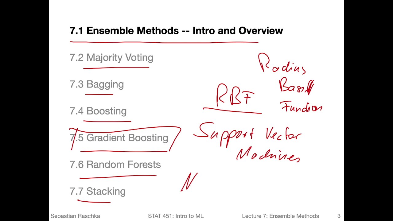
Deep dive into kernel functions (e.g., Radial Basis Function (RBF), Polynomial) and understanding the 'Kernel Trick' for non-linear decision boundaries.
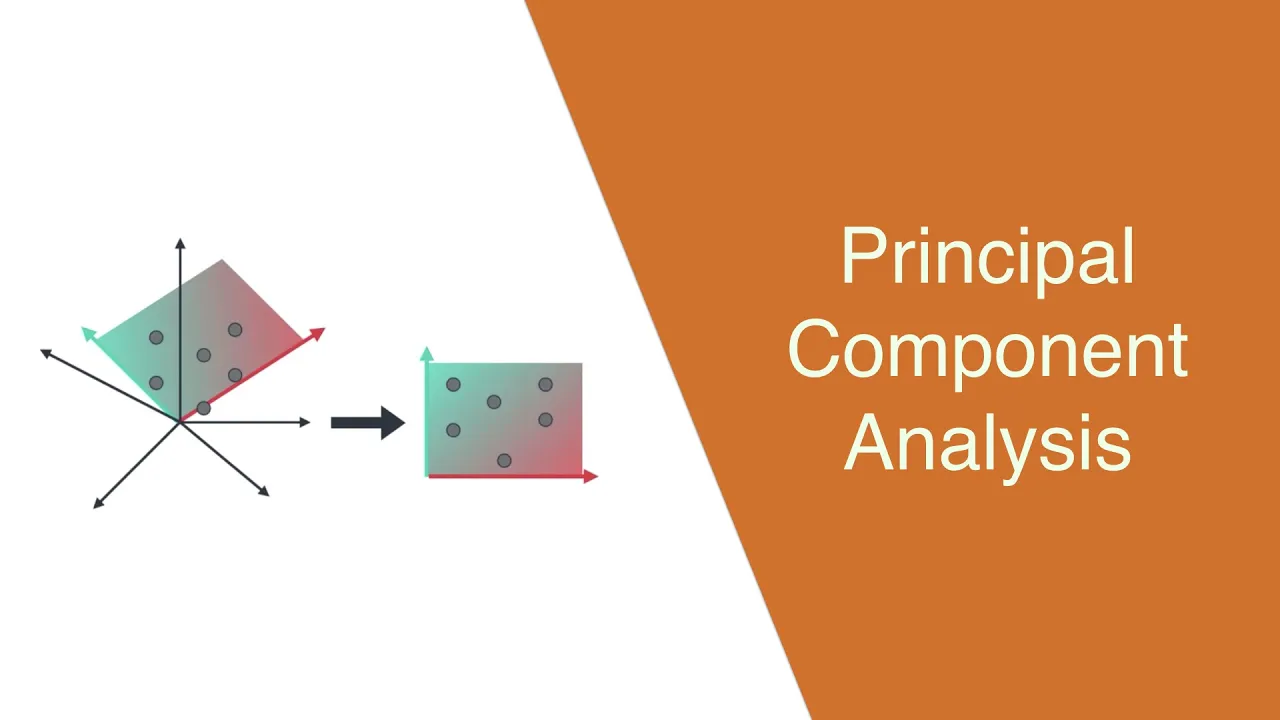
Dimensionality reduction techniques like Principal Component Analysis (PCA) to improve SVM performance on high-dimensional datasets.
Comparative analysis of SVMs against other supervised learning algorithms, such as Random Forests, Gradient Boosting, or Neural Networks, on the same datasets.
155K views4.2Klikes44:48Original Release: 2020-06-30
support vector machines quest hey yeah alright let's get started first thing I need to do is share my screen with you let's get let's get back going alright here we go oh so welcome hello I'm Josh dormer and welcome to the stack quest on support vector machines in Python from start to finish in this lesson we will build a support vector machine for classification using scikit-learn and the radial basis function our training dataset contains continuous and categorical data from the UCI machine learning repository to predict whether or not a person will default on their credit card and note throughout this jupiter notebook all these links are live so if you want to learn more about the UCI machine Rapala scheen learning repository just click on the link and there it is if you want to learn more about the data set that we're gonna be using just click on the link and there it is and you see we've got attribute information this describes the data and the data set and so so there's lots lots of sort of stuff you can click on and learn more about here is a picture of the decision service that we will create with our support vector machine we'll do this at the end but I just want to give you a sneak preview of what's gonna happen it's kind of a messy figure but it's it's what we're gonna do so let's just let's move on okay so support vector machines why would you want to do them they are one of the best machine learning algorithms out there for when getting the correct answer is a higher priority than actually understanding why you get the correct answer they work really well with relatively small data sets and they tend to work well out of the box in other words they tend to not require much optimization um so in this lesson we're gonna learn about importing data from a file we're gonna learn about missing data down sampling data formatting the data for support vector machines and we're gonna build a preliminary support vector machine then we're gonna optimize it and then we're gonna build evaluate draw and interpret a final support vector from support vector machine and we're gonna compare it to that preliminary machine mm-hmm and we're gonna see if it does better or it doesn't doesn't do better um one of the things about support vector machines is because they're great out of the box sometimes optimizing doesn't give you a huge bonus like when you're using classification trees when we did that it was night and day it was like we went from a huge tree to a prune tree and that prune tree was like infinitely better at doing classification um in contrast support vector machines tend to be pretty good out of the box so let's just see what happens note this tutorial assumes that you already know the basics of Python and are familiar with the theory behind support vector machines the radial basis function regularization cross validation and confusion matrices if not you can check out those questions by clicking these links and you're good to go also I want to strongly encourage all of you to play around with the code once you get it playing with code is the best way to learn from it there's alternative ways to do what what we want to do in this um in this Jupiter notebook and there are different ways to optimize and there's different ways there's you can even just plug in different machine learning algorithms for that matter and just see what happens there's a lot of learning that can take place by just playing around and that's when I think that's them that's the exciting part I mean this is pretty fun too so don't get me wrong ok so the very first thing we're gonna do is we're going to import the modules that will do all the work Python itself just gives us a basic programming language these modules give us extra function extra functionality to import the data clean it up and format it and then bill evaluate and draw the support vector machine note you're gonna need Python three and I've got instructions on how to install that and make sure all your modules are up to date down here we don't need to go through that because I've already got this set up on my own computer however I do want to say that we're using a jupiter notebook and as you can see jupiter notebooks are a nice way to convey combined text with code and so here is some code this is where we're importing the modules or importing pandas to load and manipulate the data and we're using it for one hot encoding there's also a numpy that we're gonna use for data manipulation we're importing menthe mat plot Lib for graphs and making things look cool and we're also importing a lot of scikit-learn stuff to do support vector machines and do confusion matrices and whatnot now when you have a jupiter notebook the way you run the code is you click somewhere in that block of code and you can either click on this play button up here to run the code there's a run menu and you can say run selected cells or on your computer there's a key combination on a Macintosh it's command or command enter or control enter on different computer systems it's different so just click the the run menu and it'll tell you what to do um so what I'm gonna do is I'm gonna click in this block of code and we're gonna run it and when you run it briefly you might have missed it there was a star there before it turned into a number one the star means that python is doing something and and at that time it was loading the modules and when it gives you a number that means it's done doing whatever it was doing so it loaded the modules pretty quickly okay now we're ready to import the data now we load the data set from the UCI machine learning repository specifically we are going to use the credit card default data set this data set will allow us to predict if someone will default on their credit card payments based on their sex age and a variety of other metrics note when pandas which is what we're going to use to read in the data when it reads in data it returns a data frame which is a lot like a spreadsheet the data are organized in rows and columns and each row can contain a mixture of text and columns excuse me text and numbers the standard variable name for a data frame is the initials DF and that's what we're gonna use here and I've got two blocks of code here one is to read in the file that we're gonna use this is a file that will be included with a cheaper notebook so you don't have to download it or anything we're gonna be using read underscore Steve CSV to read it in the file has a header row so the very first row actually it's the second second row in the data set has the header information the first row has some other kind of nonsense and I don't actually remember what it was and it's tab delimited so we're setting this separator to the tab escape sequence however you can also read this directly from the UCI machine learning repository directly you don't have to download the file first um and this is commented out so we won't be running but when you play around the code later you can feel free to play with it yourself okay so we'll load in the data and there we are we've got a number here that means we ran the code and so now that we've loaded the data into a data frame called DF we're gonna look at the first five rows using the head function um let's just run that so we've got D F dot head and that returns us the first five rows and we see that we have a bunch of columns for the variables collected for each customer the columns are ID that's just an ID number I'll limit balance is the is the is the credit limit for that customer sex is male or female education marriage age payment these these columns tell us whether or not the last payment was on time or later or how late it was there's there's one column for different months of payments so so we found just one last month's payment its it goes back six months then we have the bill amounts for the last six months last six bills and how much was paid for the last six bills and then lastly we have default payment next month this is the variable that we're going to try to predict and here I've listed the column names as well but note the last column name this one default payment next month that is a mouthful so we're gonna change it to just be default um so did they default or not um and we do that by doing data frame don't rename and we pass in the column name that we want to change and then the name we want to change it to when we set access to columns um so we're specifying that we want to change a column name lastly we're saying we want to do it in place meaning we're gonna modify this data frame that we're not gonna I'll make a copy and then save it as a new variable and then what we're gonna do is we're going to print out the next the first five rows and we're going to verify that we rename the column correctly okay so we look over here and we see that the last column name is now default and that's great that's what we wanted the other thing is this is ID column these are just random numbers that were assigned to each customer and they're not informative so we're gonna drop it so we'll do that with D F dot drop and we're specifying the ID column again this is a column and we're gonna do this in place just like we did before and we're gonna print out the first five rows to verify that we were moved the column and there it is like we've got ID up here and now we no longer have the ID so hooray we've cleaned up the columns a bit and now that we have the data in a data frame called DF we are ready to identify and deal with missing data unfortunately the biggest part of any data analysis project is making sure that the data are correctly formatted and fixing it when it is not the first part of this process is identifying and dealing with missing data missing daily data is simply a blank space or a surrogate value like n/a that indicates that we failed to collect data for one of the features for example if you forgot to ask someone's age or forgot to write it down then we would have a blank space in the data set for that person's age there are two main ways to deal with missing data we can remove the rows that contain missing data from the data set or we can impute the values that are missing and in this context impute is just a fancy way of saying we can make an educated guess about what that value should be so in this section we're gonna focus on identifying missing data in the data set first let's see it what sort of data is in each column to do that we've got our data frame and we're asking for the data type so we're going to check out the data types with the d-types command and when we run that code we see that every column is inte 64 which is good or at least it looks good because it doesn't tell us off the bat that the person mixed letters and numbers um in other words there are no na values and that suggests that maybe things are in good hands and because they didn't use character based placeholders for missing data and data frame that's just that said we should still make sure that each column contains acceptable values the list below describes what are allowed in each column and was based on the column descriptions in credit card in the on the credit card default web page so the limit balance of the credit balance or credit limit excuse me is the amount available available credit and that's an integer sex is a category we have one for male and two for female education is also a category we've got four categories for that graduate school is 1/2 equals University 3 is high school and 4 as others marriage is also a category we have one for married to for single and three for other ages and integer pay this is the these are a series of columns that tell us when the last six bills were paid negative one means on time and then we have how much after that we've got how much it's been delayed we've got bill amount pay amount and default which is a binary column that has zero for did not default and one for defaulted so we're gonna start by making sure sex only contains numbers 1 & 2 and we do that with our data frame and in square brackets we specify that we want to look at the column named sex and we've got that in single quotes and we're what we want to do is we want to look at the unique values in that column and we do that with the unique function so let's run that and we see that the unique values in this column named sex are 2 & 1 so BAM it does um now we're going to look at education to make sure it only contains 1 & 2 3 & 4 so we do the exact same thing we did before only we swapped sex with education when we run that we see that for reasons unknown in addition to the allowed numbers 1 2 3 & 4 education also contains 0 5 & 6 it is possible that 0 represents missing data and 5 & 6 represent categories not mentioned in the original specification but that's just a guess oh now we're going to look at marriage and make sure it only contains 1 2 & 3 so we do that the exact same code as before only this time we're specifying the column named marriage and like education marriage contains 0 which I'm guessing represents missing data now note this data set is part of an academic publication that is not open access it's owned by a company called Elsevier so in theory I could pay Elsevier a lot of money to get the article and find out if 0 represents missing data or not there's a good chance that the author's even didn't even mention in the article so there's a good chance that even if I paid a lot of money for the article I still wouldn't know and because this is just a demo I'm not gonna worry too much about being correct and instead we're just gonna see what happens when we treat 0 as missing data and I will give you I will say this I tried it both ways and the support vector classifier performs better when we treat zero as missing data so I at least tried it both ways and and I said well since it works better this way we'll just assume that that means missing data since scikit-learn support vector machines do not support datasets with missing values we need to figure out what to do with the zeros and the data set we can either delete these columns from the training data set or impute values for the missing data first let's see how many rows contain missing values we do that by using the Lok or location function that is associated with our data frame and what you do is you specify a sort of a logical statement that if it's true it'll return [Music] of those those specific rows that were interested and were over what we're interested in if we're interested in finding rows that have zero in the education column or and that's a logical or and an old-school computer language talk we call that a pipe the pipe character but it's a logical or so we want to eat so we want all of them we want we want all the lines in the data set where there's a zero in the education column or or there's a zero in the marriage column and we wrapped all of this up in the Len function which is short for length and so we're gonna count the number of rows that have zeros in those columns and when we run that we see that there are 68 rows that have missing values so now we're gonna count the total number of rows in the data set and we're gonna use that Len or length function just like we did before only this time we're not specifying which rows we want and when we don't specify specific rows we'd get them all and we see that there are 30,000 rows in the data set to begin with and so 68 of the 30,000 rows or less than one percent contain missing values since that still leaves us with more data than we need for a support vector machine we will remove the rows with missing values rather than try to impute their values and like I said we're gonna try to do imputing imputation in a future webinar hopefully in two months so the way we do this we select all the roads that do not contain zero in either education or marriage and the way I said that was a little awkward because we're actually going to use an and a logical and in this statement so just like before we're getting all the rows we're using this loke function to get the rows that where this logical statement is true and what we want are rows that do not have 0 in education and do not have 0 in marriage and we're gonna save all those rows that don't have zeros in education and ah and they don't have zeros in in marriage we're gonna save all those rows in a new data frame called data frame no missing all so we'll run that and since data frame no missing has 68 fewer rows in the original data frame it should only have twenty nine thousand nine hundred thirty-two rows so we're gonna count the number of rows using that length function again and there we got it hooray the math works out however we can also make sure that education no longer contains zeros by printing out the unique values this is exactly what we did before however now we're specifying data frame no missing rather than just data frame the original data set and now we see that there's no zero there and when we do the same thing for marriage we print out the unique values for marriage now we just have one two and three so BAM we have verified the data frame no missing does not contain any missing values all right and we're ready to move on to the next section where we down sample the data set so like I've said support vector machines are great with small data sets they the the data set that we used for classification trees is relatively small and support vector machines do pretty well with that data set um however uh like I said they can take a long time with large data sets and this is relatively large so we're gonna down sample both categories customers who did not default and customers that did down to a thousand each so first thing we're gonna do is we'll remind ourselves how many rows of data were working with because we remove some of them so we use the length function again and that tells us we've got twenty nine thousand nine hundred and thirty-two samples that's relatively large so we're going to down sock down sample it to a thousand of each category so the way we do that is we've created this we've already have this data frame called data frame no missing and we're specifying we want all the rows where the someone did not defaults a default is zero and we're gonna store that in a new variable called DF no default and then we're doing the same thing for the people that default it we're storing them in another data frame so we're splitting the data into two variables here one for people that default it and one for people that did not default and now what we're doing is we're down sampling the people that did not default we're using the resampled function and we're passing it the the data frame that consists of people that did not default we're setting replace to false so that means when we pull something out of there we don't and we put it in our new data frame we don't put that back in the pool of possible people that we could select again and we're saying that we want a thousand samples and we're setting the random state to 42 that's a random seed and all that does is make sure that you get the same answer that I get all and then what we're gonna do is we're gonna print out the length of this new data frame that we're creating data frame no dough no default downsampled so let's run that oh no I got there too early I didn't split the data set and a half so yeah so when you see this pink that means there that means something went wrong and instead of feeling great shame what you got to do is just got a default Deebo debug it and so let's rerun this again because before the first time I ran it I hadn't run this chunk of code first and so this data frame no default this guy did not exist but now it exists so let's see what happens and it runs and tells us we've got a thousand rows and our new data frame data frame no default downsampled now we're gonna do the exact same thing but this time we're using the people that defaulted and we're going to print out the number of rows there and there so we've got two new variables each containing a thousand rows each and now what we want to do is we want to merge them back into a single data frame and print out the total number of rows to make sure everything is hunky-dory to merge the two data frames that were created we're using this pandas function called concat which will concatenate the two two things so there we go BAM mm so now that we've taken care of the missing data we are ready to start formatting the data for making a support vector machine the first step is to split the data into two parts we're gonna have one part that contains the columns of data that we will use to make classifications and one part is going to be a column of data that contains the things we want to predict so we're gonna use the conventional notation of capital X to represent the columns of data that we will use to make classifications and we're gonna use lowercase Y to represent the thing we want to predict in this case we want to predict default whether or not someone defaulted on their payments um so here's how we're going to do that we've got our down sample data set and what we're doing is we're gonna drop the default column and we're going to copy that we're gonna store that into uppercase X and that's gonna be our set of columns that we're going to use to make predictions and then we're gonna print out the first five rows so let's do that BAM okay you'll notice we scroll over to the right we no longer have that column called default so this data set does not contain the thing we want to predict now here or we're going back or going back to that date data frame that contains the down sampled samples ah and now we're just specifying that one column default and we're making a copy of it and we're storing it in a new variable called Y and then we're gonna print out the first five rows BAM okay now we've created uppercase X which is the data we're going to use to make predictions and lowercase Y which has the data we want to predict we are ready to continue formatting x over here so that it's suitable for making a support vector machine oh okay so now we're on to one hot encoding now we have to split the data frame into two pieces uppercase X which contains okay we've already done this we've split things up now what we need to do is take a look at the variables in X and this list tells us whether the variables supposed to be an integer or a category so we see limit balance is an integer that's the credit limit sex is a category that's male or one for male two for female education has a bunch of categories 1 2 3 & 4 we've already talked about these okay so it looks like sex education marriage and pay are supposed to be categorical and they need to be modified this is because scikit-learn support vector machine support vector machines while they natively support continuous data like limit balance and age they do not natively support categorical data like marriage which contains three different categories thus in order to use the categorical data with scikit-learn support vector machines we have to use a trick that converts the column of categorical data into multiple columns of binary values and this trick is called one hot encoding um so at this point you may be wondering what's wrong with treating categorical data like it's continuous so to answer that question let's look at an example for the marriage columns we have three options one married to single and three other if we treated those values one two and three like continuous data then we would assume that three which means other is more similar to two which means single than it is to 1 which means married and that means the support vector machine would be more likely to cluster people with threes and twos together than people with 3s and ones together and in contrast if we treat these numbers like categorical data then we will treat each one as a separate category that is no more or less similar to any of the other categories thus the likelihood of clustering people with twos and threes is the same as clustering threes and ones and that approach is more reasonable note I have a huge treatise on different ways to do one hot encoding there's two very common ways to do it there's a there's a function called column transformer from scikit-learn and there's a function called get dummies from pandas because I believe that get dummies is bed it better for teaching how one hot and coding works we're gonna use it however just know there's alternatives and you should definitely read this description at your leisure to learn about the pros and cons of these two different approaches okay first before we commit to converting columns with one hot and coding I just want to show you what happens when we convert marriage without saving the results so to make this easy to see we're gonna use get dummies get dummies as a Panda function and so we pass it X capital X that's the columns that we want to transform and we specify the columns that we want to transform for this demonstration we're just gonna transform marriage and then we're gonna print out the first five rows to see what it did okay scroll over here and you'll see that on the left side of the data frame are the columns that we did not touch and on the right side we've got three columns for marriage we used to just have one that contained three values now we have three columns and each one contains a 0 and a 1 1 in this column marriage 1 there's a 1 if there was a 1 in the original marriage column there and a 0 otherwise for marriage - there's a 0 if where there's a 1 if they originally had a a 2 in the marriage column and a 0 otherwise and marriage 3 is 1 if they originally had a 3 in the original column zero otherwise so that is how one hot encoding works okay now we're gonna do it for all of the categorical um columns and then we're gonna print out the first five rows just to see what it looks like alright so here is our new data frame we've got a dot dot dot specifying that some columns are not shown but you see that hey these columns have all been converted into new columns so double bam the last part of formatting the data for a support vector machine is to Center and scale the data um the radial basis function that we're going to use assumes that the data are centered in scale scaled so in other words each column should have a mean of 0 and a standard deviation of 1 so what we're gonna do is first what we're gonna do is we're gonna split the data into training and test data sets so we're using train tests split again we're setting the random state so that you could reproduce what I've got we're passing it in X encoded that's the one haunted coded X these columns over here that are that are gonna make the predictions and we're passing em Y that's the thing we want to predict and we're creating X train X test Y train and why test I believe the default setting is for 70% of the data to go into the training data set and 30% to go into testing don't quote me on that I just believe that's the case after we do that we are scaling the data sets using the scale function now right long um now we're gonna talk about building a preliminary support vector machine um we've done a lot of stuff we've almost been a whole hour just formatting data and now we're finally getting to the good part the way we do that is we call SVC for support vector classifier we set the random state to 42 and what this does is it kind of makes an untrained shell of a support vector classifier the next step and we're saving that shell as classifier underscore support vector machine the next step is to call fit using that shell and so what we're doing is we're fitting it or we're training it on the training data so we've got X train scale and y train oh and we know we don't scale y train because that's just 0 on one and my brain was left my head for a second so anyway so that's correct and we run it and it just prints out the support vector classifier plus the default settings that it has and now that we've trained the classifier we can see how it performs with confusion matrix and we're going to use the test data set we're passing in we're using plot confusion matrix for PLAs passing in our trained support vector machine and we're passing in the test X data set and a test Y and below we're just formatting it so it looks pretty so here is our class here's our confusion matrix it did all right it did not do great of the 257 people that did not default 79 percent were correctly classified of the 243 people in this row that defaulted 61% were correctly classified so the support vector machine was not awesome so we're going to try to improve that using cross-validation to optimize the parameters to optimize the parameters we're gonna use grid search cross-validation or grid search CV and when we optimize a support vector machine it's all about finding the best value for gamma and potentially the regularization parameter C so what we're gonna do is when we use grid search CV we specify the parameters that we want to try in this you know in a matrix um and so we've got this is the parameter C which is the regularization parameter and we're gonna try these values um note the regularization parameter Scott to be greater than zero oh and there's gamma and these are the values were specifying for gamma in theory we could try other kernels if we wanted to and specify those as well that ends up taking a long time so we're just gonna stick with the radial basis function typically it gives us the best performance okay so then we run grid search C V and we pass in the shell of a support vector classifier we pass in the parameters the C V is the number of folds of Kraft cross-validation we want to do then we pass in the scoring metric that we want to use there are lots of options and I tried a bunch of them and true to its word support vector machines tend to be good out of the box and I was trying to find a metric that would give us huge improvements and I wasn't able to find one but you can uncomment these and try different metrics there's even more I'm using here um anyways um this Wilkin will return something we're saving in a variable called optimal parameters and then what we do is we run the cross-validation on the parameter values by running optimal values fit using the training data set and then we're going to print out the optimal best parameters so we'll do that this is gonna take a little long you'll see this a star here that means a Python is hard at work doing cross-validation for us when that turns into a number it'll print out the output down here and this is one of the reasons why we downscaled the dataset we went from 30,000 rows to just 2,000 and it still took a little bit of time I mean we're not talking hours but it still took a little bit of time these are the optimal parameters by the way we're done running we've got a number here oh and we can see that the ideal value for C because that's a literation is 100 which means that we will use regularization and the ideal value for Gamma is 0.001 so now we're ready to build evaluate draw and interpret the final support vector machine so now we're doing exactly what we did before however this time we're specifying C equals 100 and gamma equals 0.001 and then we are so that creates the shell and then we train it using the training data so we'll run that BAM and now we're going to print out a new confusion matrix with our new support vector machine and we're going to run that and here is our all put and these are the results the optimized support vector machine and they are just a little bit better than before for more people or correctly classified as not defaulting however one person was incorrectly classified as defaulting so that mean depending on how you want it depending on whether or not it's more important classify these people or these people we may have improved or we may have slightly gotten worse but that just tells you again that support vector machines are pretty good out of the box optimization didn't help us that much okay now we can actually draw what the decision boundary is um this is a pretty complicated procedure and at best it is an approximation of of what is really going on and we can quantify how good that approximation is various ways that we can quantify how good that approximation is going to be and we'll go over that really quickly the first thing we're gonna do though is we're gonna look at see how many columns in our our data set so we've got 24 columns in our data set and this is a problem because that means it would require a 24 dimensional graph um or maybe even more because we're using the radial basis function and that operates in infinite dimensions and since we can't draw an infinite dimension we have to do data we have to collapse the data into two dimensions so we can draw a picture of that we're gonna use principle component analysis to do that and if you don't know what principal component analysis is right now just know that what we're doing is we're taking those 24 columns and we're gonna shrink them down to two um and then so this is the code for doing that and we're also gonna plot what's called a scree plot and this scree plot tells us how good this approximation of the true classifier is the what we would like is for the first two principal components the first two columns here to be much taller than all the rest and that means that those first two components can be or those those two columns that we're going to use for our new data set would accurately reflect the original data in this case we don't see that what we see is that the first principal component the first column is is stands on its own that's good that's what we want however the second one is just barely taller than the others and that's not good and that tells us that this approximation is not going to be great um that said I'm also including in this in the in the email I'm going to send out you're going to be able to download how to do support vector machines with this different this with this heart date heart disease data set and in that case the image is better and actually classification in general is better so it's so baked sure you run through both of these because you'll get different results and you'll see then that how to decide when it's going to be a good sort of collapsing of data and when it's not um the next data is pretty complicated next data code chunk however just know that what we're doing is we're retraining and re optimizing a support vector machine on just those two columns that we collapse the data down to we run that this we're doing cross-validation so this is gonna take a minute or two um and while this is running I will address this going question yes we are recording this as a video and I'll put it online and you'll be able to access this later on it your leisure and I'll email you the link okay so it's done running we've got optimal grammars notice we've got different optimal parameters and before that's because we're actually using a different data set instead of all 24 columns we're just using two now and that's you know like I said we're approximating what we did with the 24 columns here this is when we're actually drawing that decision boundary lots of code but also very well commented so you can go through this at your leisure right right now we're just gonna run it really quickly and we're going to look at our picture and here it is kind of a mess but kind of what we expected because the first two principal components which form the x and y axis of this graph don't do a great job capturing sort of all the variation that's in the data and we knew that going into this so when we get it kind of a messy thing it's what it is okay so BAM the pink part of this graph represents the decision area where we if someone falls in there would classify them as not defaulted the yellow part is where we'll classify people as defaulted red dots are from the training data set that are known to have defaulted so this person is known to be defaulted they landed there the green dots are people that are Oh red is no default and yes as default anyways that's how to interpret this graph you can read more about it here okay so in conclusion we've loaded data from a data file identified and dealt with missing data we down sampled the data we formatted the data for a support vector machine using one hot encoding we built a support vector machine for classification we optimize the support vector machine using cross-validation we mainly built drew interpreted and evaluated the final support vector machine and that gives us a triple BAM hooray we've made it to the end
Up Next

13:21
Science in Islam: The Mu'tazila & Free Will | Historical Analysis
@CaspianReport
164.9K views•2017-05-01

12:54
Triumph of Orthodoxy Icon: Byzantine Art & History Explained
@BenCallan
2.1K views•2024-08-06

9:49
FastAPI vs Flask vs Django: Choosing the Right Python Web Framework
@TechWithTim
302.5K views•2024-05-26

1:42
Game of Thrones Opening Credits: A Cinematic Analysis
@gameofthrones
46.3M views•2011-04-18
Related Study Plans & Knowledge Roadmaps
Structured learning paths in General & Interdisciplinary Studies
general-studies
Elevator Engineering: History, Physics & Cities
01From Hoists to Safety Brakes: The Dawn of Vertical Lift
02Hydraulic vs. Traction: The Engineering Physics of Elevators
03Modern Speed, Safety, and Algorithms
+ 2 more learning modules
12h5 modules
Explore Roadmap
general-studies
Rubber: Material Science, History & Geopolitics
01Origins of Natural Rubber & Mesoamerican History
02The Chemistry of Natural Rubber & Vulcanization
03The Geopolitics of the Rubber Boom & Colonization
+ 2 more learning modules
12h5 modules
Explore Roadmap
general-studies
Containerization: Evolution, Logistics & Trade
01Ancient Trade & Bulk Cargo: Amphorae to Barrels
02The Industrial Revolution & Cardboard Packaging
03The Containerization Revolution: Malcom McLean
+ 2 more learning modules
12h5 modules
Explore Roadmap
general-studies
Textile Tech: Evolution, Labor & Global Impact
01Pre-Industrial Textiles: Handloom & Cottage Industry
02Mechanization: The Spinning Jenny to the Power Loom
03The Factory System & Global Labor Transformation
+ 2 more learning modules
10h5 modules
Explore Roadmap