Aerosol Optical Properties Uncertainty from Size Distribution Data

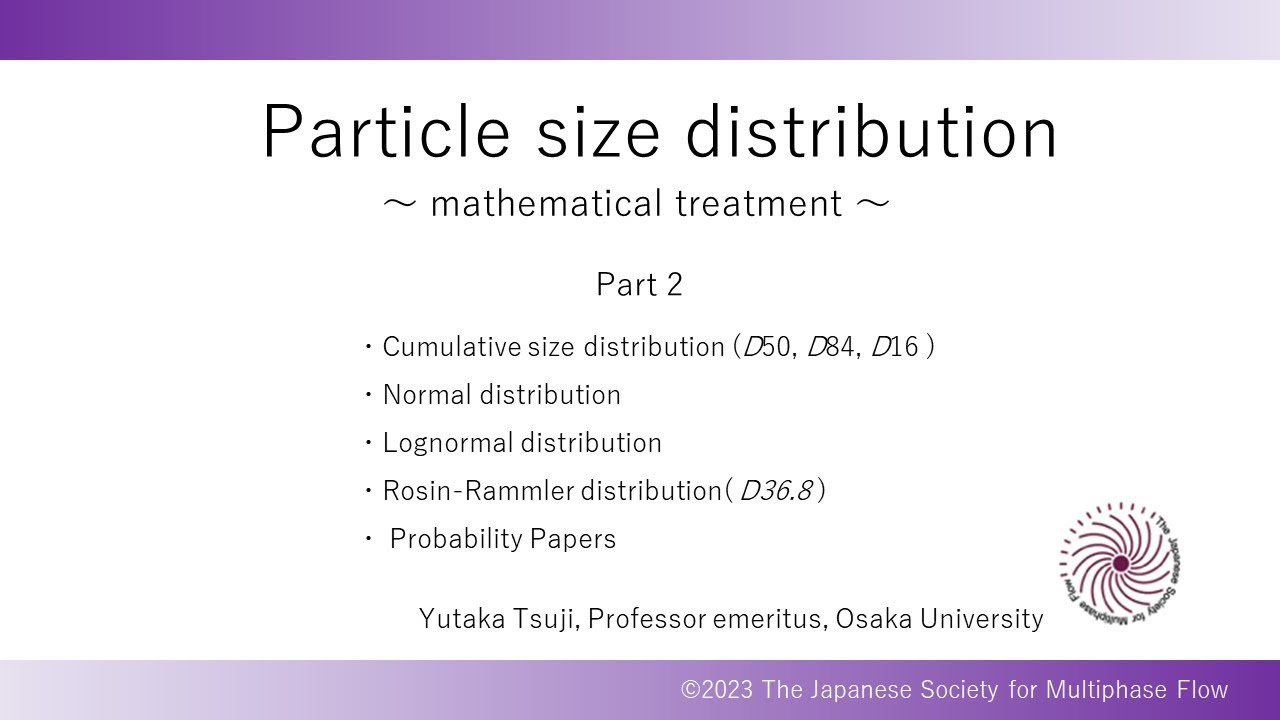
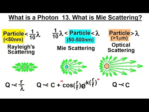
[00:00:01]hi my name is Amy Sullivan and I'm the current vice president of Tri it's my pleasure to welcome you to the 27th in our monthly series of as&t lectures this is a new Initiative for triple being supported by the Freelander memorial fund so with these lectures we hope to highlight the amazing research tapping our community um to tie our Journal other activities and also give us a chance to all come together outside of the annual conference so each month the editors of as&t select a high impact Journal article to be presented by authors these lectures are being recorded and will be later posted to Tri AR's YouTube channel which you can access from the tri AR website under the events tab in addition these lectures are being hosted by one of our student chapters and so I want to thank you all for joining us and everyone who's help to make these happen and with that I'll turn it over to our Student Chapter from the University of Maryland College Park to get it started thanks hi everyone my name is nahen I am the current Student Chapter president of Tri AR for University of Maryland College Park and today I have the honor and pleasure of introducing Dr Hogan Tel um Dr Tel is a research scientist at Noah's Global monitoring laboratory and sear at the University of Colorado Boulder um he obtained his PhD in solid state physics from the Technical University of Berlin in Germany and embarked on his Us Journey as a postto fellow at Los Alamos National Laboratory in 2010 transitioning into into aerosol into atmospheric sciences 2013 uh Dr T initially focused on aerosols from the perspective of instrument development and later he increasingly shifted his attention to data product development and Analysis of long-term data records while maintaining his dedication to aerosols today he will be discussing um aerosol Optical properties calculated from size distribution measurements so I will hand it over to Dr T yeah hello everyone and uh thanks for uh yeah coming so plentiful and I want to thank first of course for this nice introduction and um I want to thank the editors for choosing my work uh to yeah so I can present it here and um to such a broad audience so let me share my screen um okay so today I'm going to talk about um uh aerosol Optical properties and how to derive those from um size distribution measurement and what the uncertainties are and that are involved in such a effort and um I don't know how it is for you but uncertainty study of always uh triggers this involuntary yarn in in me um or at least it used to be but um this study actually changed my mind and I had a lot of fun um digging into all those uh instruments the techniques the um and the the methods and playing with new models so I hope I'm able to uh convey this the joy I had during this study um so I will start with a with an introduction to the whole topic um and then I will introduce you to all the key uncertainties in including the instrumental uncertainties uh the limitations due to the theory and this case me Theory and then also how the different microphysical properties of our aerosols are affecting measurements as well as um the calculations um then I will um describe how propagate those uncertainties using um The Mont Caro method and um then finally of course discuss the results so why should we all be interested in aerosol um Optical properties and the main reason is of course the aerosol direct effect on the earth radiative budget here um shown on the oops there um here Illustrated on the right where we have the part that is uh scattered back back into space the part that is absorbed and then also of course how much makes it to the ground and there are three aerosol properties that are necessary to describe this um aerosol direct effect which are the scattering coefficient and which describes the overall scattering so here on the bottom I show just for a single particle how the scattering might look like so we have the the all the scattering that's a SC which is described by the scattering coefficient then the asymmetry parameter which um is more um describing the directionality which is nicely uh seen here and which of course then will help us uh understand how much is scattered forward um and reaching the ground or how much is getting back into space and then the last uh property is the single scattering albo which describes the absorption of the the aerosol particles but today I will only focus on one which is the scatter coefficient so um I will ignore all the other ones um in principle you can measure those properties directly um using nephelometers and aoms um and that is done all over the world on a um routine basis for example um the Noah uh Federal Federated aerosol Network which we which is run or partially run by colleagues from my group and which does these type of measurements but alternatively you can also um derive your Optical properties from more from the bottom up where you use the microphysical properties of your aerosols and so what you would do is you collect somehow your microphysical properties um like particle size distribution refractive index particle shape but um you name it could be many more and then you use some type of a theory and model your to calculate your Optical properties and um but why would you do that the main re or like one of the reasons is of course because when you have those um microphysical proper properties you can evolve your aerosol and um physically as well as chemically and that is of course important for modeling and indeed uh the modern uh General circulation models climate models um are increasingly in into using microphysical properties to propagate the aerosols um and in turn of course also propagate the the radiative effect of those uh properties so if you want to engage in this path then you of course want to make sure that you understand the whole process correctly so usually this is done in closure studies so you you um you have um on the one hand you have an observation uh or you have two sets of observations on the one hand you would have in our case the Aeros Optical properties on the other hand you have the microphysical properties and then you have your theoretical model and you want to make sure that they are the same um and I it was such a study that made me um do this work and um in in that study I struggled to get them to agree within the previously assumed uncertainties um and it regularly and um excessively uh overestimated or exceeded those um confidence intervals so um and also there were almost 20 years old those studies so I thought it's time for a for a new approach with a more recent um like more recent Publications that came out so um so I want to set now a little bit the scene of this study and I want to for that I go back to the slide I just s um showed earlier and want to give it a little bit of um reality check so usually um you do not measure all that many um aerosol microphysical properties the most common one is the particle distribution but the other ones are rarely observed and they often have large uncertainties and uh especially if you do not have the any information on the particle shape then you might as well use a rather a simple um theoretical model which is usually the me Theory um to describe your Optical properties and um so this brings me to the first um boundary of this work or constraint is I will discuss uncertainties resulting from using me Theory to calculate scattering and only from size Fusion measurements which which is the most common or a very common thing uh that is found in the literature uh another um con confinement um is the um the location aerosols are known to be very variable not just in time but also um with respect to the geographic location and um so instead of uh it's B basically it would be very hard to do that uh to do a study like this that is valid everywhere so I pick a particular location which is the the arms the atmospheric radiation measurement a southern Great Plain side which you can see on the map on the right is located in um Central Northern Oklahoma and the reason why I pick this um this particular site is for one they a lot of different uh uh instrumentations that are run on a long-term basis um and also that's a place where I wanted to do the closure study of course um so um the the if you want to measure size distribution there's basically not a single instrument that can measure the entire or let's call it for this purpose relevant for optical properties and the size distribution so you have to combine different observations and a very common combination is the which is also present at SGP is the scanning Mobility particle Sizer and the aerodynamic particle Sizer and where the um the snps the scanning Mobility particle Sizer measures uh in this particular case at SGP up to 750 nanometers and the aps um is measuring for um above that and um all right and and what I will do is I use this particular size distribution throughout the whole study so this is my Exemplar exemplary um size distribution and you will see it quite a lot so it is the average over the year um of 2012 measured as as measured at SGP with those two instruments um and then I will do a further um set a further boundary and that is um I assume that the snps it's actually a very important simplification for this study and that is that the snps measures the accumulation mode particles and the aps is measuring the cause mode particles and um why this is so important is um first of all accumulation mode and cause mode particles have different Origins and therefore they have different microphysical properties and um and therefore this simplifies this study a lot if I can now treat the um the smnps measured accumulation mode on one side and the um APS measured uh cuse mode particles on the other side independently uh it's a nice simplification and it has another um benefit that uh that is that for this particular study um I can oh yeah I only will present the snps part but um I forgot I wanted to of course first motivate why this is a good choice a good approximation and um as you can see on the right in the size distribution I added now the contribution of the the cause mode here and the accumulation mode um given by these stashed lines and um while in the number concentration size distribution representation it might not be that obvious that this is a good um motivation to split it here when you now calculate the scattering from for the different as a function of the diameter then you end up with this Orange um picture here um a second with a orange graph and you can I again showed the the contributions of the accumulation mod and the cuse mode by these dashed lines and now it it is I think pretty convincing that um that to split the size distribution at um this uh diameter um but at 750 NM and there's only little contribution of the accumulation mode um to the larger particles to the um APS measured side and the other way around okay so as I said I will only focus on the snps side today and um that is uh uh very convenient because I would otherwise most likely run out of time and also I there's a lot of um re uh repetitiveness um a lot of uh I would have to repeat myself a lot so um that's not very conducive to the attentiveness of the audience I I assume so and the the last part um of the introduction is the the uncertainty propagation that I will use in this study and that is the the Monte Carlo approach more a Brute Force approach the reason why I use that over a more classical approach is um that the classical approach is very convenient for simple problems but the more complex a problem be um gets um the the less adequate um it is and also and the more adequate such a Mont Caro approach will be and um so the way the Mont Caro approach works is um you instead of using the uncertainties um for all your variables that that are uncertainty that are carrying uncertainty you now um get a distribution a prob ility distribution shown here on top for each of these variables these distributions are of course um according to their uncertainties but also they they have more information they they don't need to be normal distributed for like for for this uh first for the X1 here they can also be uniform distributed or um uh like uh log normal or other um yeah other distrib bution so in our case of course those uh those parameters on top would be like instrument uncertainties uncertainties due to changes in the microf physical Pro properties and so on and then in the next step you take always one set from these distributions one random set and you apply it to a function and that function needs to uh the the the dependent variable that you get from this function is of course the function the the the of interest in this case it would be the um scattering coefficient and then when you um repeatedly take random sets of these variables and feed it into your model then eventually you will will end up with a distribution of your dependent variable a scattering coefficient and that uh then you can do your statistical analysis on including um your uncertainty estimate okay so in the first in the next part of my presentation I will now focus on how to derive all those and distributions starting with um the part the instrument part so um I obviously will only discuss the smps because the aps uh I skipped that part for um reason of time and um yeah so the mobility SC uh the the scanning Mobility particle Sizer is uh the the general principle of it is um it uh how particles are drifting uh in an electric field so charge particles obviously and um the way that is achieved is you you start with um introducing some uh um charge Distribution on your particles which is done with these neutralizers and then it enters the instrument the main part the instruments and then when it enters into the electric field um all these charged particles are getting are starting to drift and um only particles that drift by a very particular um amount will then um enter these slits and eventually get counted with a condensation particle counter so the amount that they drift is um a function of uh the voltage and electromobility sh in this function then the electromobility is a function of the diameter and uh so the particle diameter and the number of charges on the particle and since we know a little bit about the the partic the number of charges based on our what our neutralizer is doing we can then um get the diameter as a function of voltage and to get the size distribution we would only um scan through the voltage and then get our size distribution after applying a rather sophisticated transfer function so it's not as simple as I as the three um equations here might suggest and um you can of course imagine many sources of uncertainty in such a complex system and it would be quite a fee to get a uh to qu get a quantitative meaningful value out of um out of this but luckily there is an alternative and that is a multi-instrument intercomparison studies and which in fact uh have been conducted um and um and by by this group here on the left um sorry there's a reference here on the left with probably the longest um title I have ever seen um that um on the top right I'm showing some of those results that are presented in in this paper and um so it chose the size distribution in particular um the volume distribution here um of these seven different snps uh instruments and you can immediately see that especially for the larger diameters um these they they deviate by quite a lot and um as you will see later it's uh quite important to not just now take the average of all of this and assume that to be the uncertainty um it is important to consider the size dependence of this um deviation and um so how we do it is we we take the mean of all those uh graphs here and assume that that is the real size distribution so we assume that that has a counting efficiency of one so we we normalize all those uh graphs by the mean the mean and then the distribution of all those graphs around the mean are then our counting efficiency and how we apply that then in the Monte Carlo approaches we simply take a standard normal distribution like shown here and then if we pick one of those values let's say one then we would take the size dependent counting efficiency that is according to uh to one standard deviation and apply that um the the um this paper was also handling dealing with a sizing precision and uh which was not size dependent so they we just use the the relative standard deviation that was reported and uh use the according um normal distribution for our probability distribution um so in addition to these more intrinsic instrument uncertainties um we can also unfortunately assume uncertainties due to imperfections of our particles in particular um we have to assume that particles are not always spherical and uh and the electromobility is in fact affected by the shape of the particles um actually most in most measurements are one way or the other affected by um by the by the shape of the particles and therefore um to get around that to um somehow describe that you you would use the equivalent diameter so the snps is not measuring just the diameter but the mobility equivalent diameter and um what we will use later for our Optical property calculations for that we will need the volume equivalent diameter and um there there luckily there's a relationship between these two which is shown here on the right where you can describe the the the mobility diameter as a function of the volume diameter if you consider um the shape of the particle which is here um the dynamic shape factor it's uh in given by She and then um which you can then Express as the geometric shape factor which we will need for the optical um property calculations which is given by uh Fe and um yeah just to to to um say what the this geometric shape factor is it is basically the ratio between um the um first of all it assumes that the that you approach the approximate your particles as spheroids like these Pro um oplate and prolate spheroids and then the geometric shape factor is given by the ratio between the longer axis and the shorter axis and minus one so and how we now would uh consider that in our Mont Carlo approach is first we have to find of course a distribution of this and um you um yeah typically uh the accumulation mode particles are usually considered spherical and there's only a handful of uh observations or studies that study and the shape of those particles and they found that they're actually not all that spherical and they um they as you can see here on the on the left they they can have quite a lot of different shapes and they estimate um the airity aspher asphericity and the the particle shape factor to vary between minus 2.4 and four uh 2.4 which um corresponds roughly with um a ratio of 1 to three they also found that the distribution is not a normal distribution but rather res resembl such a a uniform distribution okay so much about the instruments um in the next uh part of the talk I will um I will talk about how to uh calculate the opt Optical properties from this and and um what the sources for uncertainties are here and um so let's remember I that I'm dealing with me Theory like what are the uncertainties from um when you use me Theory and so the definition or the shortest definition of the Mii theory is um that the Mii theory is a mathematical description of how light is scattered by uniform spherical particle so we already see that we will most likely run into an issue here because U we I already mentioned that particles are not that spherical and um but let's first discuss how how you would use me Theory to get your scattering coefficient so on the top right I'm showing um the scattering cross-section of particles as a function of particle diameter and um what you get is this um often referred to as a mi curve then in the next step you would use that Mi curve and convolve it with a size distribution and um what then gives you this scattering coefficient distribution and then if you just uh integrate over the scattering coefficient distribution you get your scattering crosssection and um when it uh comes to our uncertainties when I go back here to the top um you can describe the Mi curve as a function of the diameter we already talked about the uncertainties of our diameter measurements so that's dealt with but it's also a function of the refractive index and the wavelength so for the wavelength we only use the 550 nanometers and keep that fixed but um we can expect uncertainties because of V variability in the the refra index the real as well as the imaginary part and um this is a measurement that is not particularly often done um and also um if it is done then it's pretty uncertain um here on the right I'm just showing how the me curve is affected by the um refractive index by the real part of the refractive index you might notice that the smaller diameters are more effective than the larger ones where um those three graphs are collapsing almost okay so how do we get our expected um probability distribution our uncertainty for um the real part of the refractive index and this can be done uh with uh chemical composition measurements or based on chemical composition measurements luckily at SGP um there is the this ACSM the aerosol chemical speciation monitor which measured during the year of 2012 and um the the the acms is measuring ion concentrations and you can use those to estimate Electro electrolyte concentrations and you can use those to estimate your refractive index just the real part though and um so we did that for year worth of data and then um looked at what the variability the um the probability distribution um looks like and it and it is shown down here which is a normal distribution that is centered around 1.5 and when it comes to the um the imagin imaginary part of the refractive index um we have to use a different instrument and uh there's another instrument at SGP that is done that is uh measuring on a routine basis there which is the athl ometer I mentioned it earlier it's a it's a rather um simple principle you just run your um aerosol through a little filter a filter like shown on the right here and then as more and more aerosols or absorbing aerosols are depositing on the filter you will see um a slow darkening of of your filter and based on this darkening you can estimate the absorption if you then also consider the size distribution and the scattering coefficient that are measured then you can estimate the refractive the imaginary part of the refractive index which we again did for an extended time and uh which resulted in this probability distribution you can see down here here um note that this is a loog normal distribution which we found and it is centered about 0.01 013 um and then as I mentioned earlier we are running into this issue that the me theory is assuming spherical particles and our particles are not uh are probably not spherical so um we we are violating that assumption and the only way to get around this um is to use a more sophisticated Theory so what with the theory of our choice is the transition Matrix method and um the difference now is to to the me theory is that we are now um considering the oade and prolate spheroids instead of um spheres um and also they they need to be randomly oriented by the way the transition Matrix method is not necessarily um you can use arbitrary shapes you don't have to use oplates but and prolates but this is an approximation that um makes the these calculations reasonable the computational um effort so on the right I'm showing again the the me uh curve here on the top and then on the bottom I'm showing the result from The t- Matrix calculation um the these results are now normalized to the results for the sphere so basically um I normalize this by a curve that looks identical to this and therefore at one this is a spheroid axis ratio at one where we has have spherical particles and we everything is is one and then um everything around it is the deviation from that and you can see that um the dev ation can be quite substantial for example um here where we have a ratio of what is that four and five we get uh we get a ratio to the um the spherical particles of three so um that's quite substantial and of course we now don't um plot that as a function of diameter but as a function of volume equivalent diameter so we do not uh need to develop another um distribution here and we of course for these um aspheric uh properties we use the very same distribution um like the one we used above for the measurements okay this brings me now to the um to the mon Caro approach I will start with the um how the model works and then we'll apply all those um random variables from our probability distributions so um on this picture I now will present the function part here of the monal model and um I'm starting with the particle size distribution it's again the same I showed earlier um and in the first step now I will take a a random value of uh the the the diameter precision and just shift um the the the size distribution accordingly in the second step I I take a value from this uh standard normal distribution and uh apply accordingly a counting efficiency which is just scaling our size distribution then in the next step I take that already changed size distribution and convert it from our um our Mobility equivalent diameter to the volume equivalent diameter um using a particular shape that I plug into this formula which is um effectively again just a shift of along the diameter axis and the resulting size distribution then I pluck into the T Matrix calculation which in addition um take now values from our imaginary and real part of the refractive index and um from the aspher asphericity again and it's important I of course have to use the very same value here of the ace Verity as the one I used earlier when I did the conversion from um Mobility equivalent diameter to volume equivalent diameter and um that gives me then the result so here just um a brief repeat um I have all those different uh probability distributions and now I I take r random values of each of those plug it into my model then I get one Val value for the scattering coefficients and then I do that thousands of times and eventually I get a distribution for my scattering cross-section which is now my final one of my final results and this from this I can um derive my confidence interval and um um so first of all is this confidence this distribution is a loog normal distribution um so we expect the confidence interval to be asymmetric around it and the confidence interval if we take the 95% confidence interval or the two zigma then we end up with Min minus 50% to plus 100% roughly which is of course significantly larger than any of the previously um uh assumed estimates and now I'm getting back to the also to the aps to the cause mode part I just want to show you the results even though I did not introduce any of the um the uncertainties involved and um first of all while all those distributions look pretty similar they are quite different for example the asphericity is twice as big because it is well known that uh Cosmo particles are um more aspheric um then the reflective index is quite a bit larger and also we have one additional parameter that we have to consider which is a density okay so I do the same thing thousands of different combinations of all those parameters give me my um my final probability distribution my uncertainty for the scattering coefficient and it looks almost identical so now I have on the bottom is for the cuse mode um so it's a again minus 50 roughly to plus 100% And um if we now add the two together to get our overall uncertainty we expect a little bit of smaller value um because those are two independent uh um parameters and we we still end up with minus 40 to plus 70% um confidence interval which is still significantly larger than the previous uh 20 plus - 20% so while this is by itself of course um already an interesting result and what would be even more informative is if you look at what what of which of our uncertainties contribute to the most to these overall uncertainties and um the nice thing about the monteal approach is you end up with this vast amount of values these this huge parameter space and you can now model that just to get a um differentiable um function or description of it and then you can take partial dependency so I've done that using um a um generalized additive models um which is a a quite convenient tool to do this and um you will recognize all these plots here again our um parameter the probability distributions in Gray and in addition I now give in these blue lines our partial dependencies or our sensitivities and the the steeper those lines are the more sensitive is the overall um uncertainty on on this parameter and to visualize this to to make it more apparent I now convol convolved the um our probability um dist utions with that sensitivity so all those blue areas you can see in all those plots are now giving you an idea of how much this uncertainty this the the uncertainty of this parameter contributed to the overall uncertainty and there are two that um Stand Out significantly and that is of course here the counting efficiency and the ace veracity and it's the same thing for the C mode by the way and with again it's accounting efficiency and the ace vericity even though the ace vericity is twice as big for for the co mode and also the counting efficiency I mean the whole instrument is a different instrument still it's the same picture um so I want to just address those two uncertainties and um why they are so big or what could be done about it and um when comes to the counting efficiency it's a very uncertain uh coincidence uh that why that is so huge especially for the snps and that is better understood if you look again at the counting efficiency as a function of diameter and um so if I now plot the again the scattering coefficient as a function of diameter then you will see that a particular for the co for the accumulation mode and now most of the the light that is scattered coincides with this increased uh counting efficiency uncertainty which is quite unfortunate and while it doesn't look as bad for the aps especially the the peak years coincides actually with a um with this minimum um still a lot uh is of course Within These enhanced accounting efficiency uncertainties so a potential solu solution for that would be to use a different measurement for example Optical particle sizes they are known to work well in this regime but you still would want to do of course a similar uncertainty study to be sure that it is really better um then um another thing is of course I mean that's easier said than done that um maybe some some of the instrument developers could focus a little bit more on this size range because I think a lot of focus is actually on the smaller diameters because it's more relevant to chemistry but um yeah if you hear this please concentrate more on this size range it's more important for optical properties and then the other one that is for aity um yeah that's of course um a hard one but I think one reason why this is so big is that there's just not enough uh measurements not enough constraints of these values so if if just more measurements would be done um with respect to these um to the asphericity then we might be might find that it's actually more spherical than we than these few studies um showed in lab and um lab environment so um so I think just more observations would be great and would would help and then another thing is that because of these equivalent diameters you could if you overlap a lot of different measurement techniques there is a way to derive and gain information on the particle shapes so that would also be helpful okay this brings me to my summary I presented a uncertainty study of uh um ELO Optical properties that were derived from sition observations um under the use of me Theory I discussed um all the involved uncertainties uh including the instrument uncertainty but also how aerosol microphysical properties um affected our measurements and then also how those microphysical properties affected um the um the calculations of our Optical properties so um then I introduced The Mont Carlo uncertainty propagation and finally found that the scattering coefficient confidence interval need to be sign significantly larger than what was um previously estimated and then I also identified that the counting efficiency and the particle shape are the main culprits uh to our uner overall uncertainty and with that I want to thank you all for for attending for your attention thank you Dr Tel that was an incredible uh incredible talk um I learned a lot more um about Monte Carlo as well as its applications to things like you know these properties um we have time for questions uh so if anyone would like to ask a question feel free to unmute or drop it in the chat uh can I ask a question yes okay first of all thank you very much haen for this wonderful lecture of course it was quite interesting for uh the people who are working in the uh specifically in atmospheric environment atmospheric aerosols field so Al my question is uh of course uh these uh detailed uncertainty studies are associated with these scattering from the Aerosoles um uh in comparison to the uh studies you have U made with these me Theory and so uh but the uh these uh these studies are quite important when you are using these filter based method for example you have you already mentioned this eomer right however the people who are dealing with photoacoustics in which this scattering uh actually does not participate it and the source of pment and the other Optical properties uh they are depend they are dependent upon the aerosol absorption and uh their correlation with the size distribution so my question is is this kind of Monte Carlo simulations are good for the uh absorption uncertainities as well I mean in principle you can apply it to any type of propagation uh uncertainty propag so you yeah it's a it's a it's a general uncertainty propagation study you can apply it to everything it's it it is more about how you how carefully you choose your distributions and how um sophisticated you make your model that you use in the Mont Caro approach so what you're referring to I mean I I I I think I um I mentioned um what you are referring to um on this slide I assume and um I did a simplified um approach here but if you want to do it more uh th Thor thorough then you could just do a monal just for that part by itself of course I don't know does it answer your question yeah yeah of course thank you so much okay thanks uh there's someone with their ra hand raised Simone hi very nice talk thank you um my question is uh obviously you took a lot of data I was just trying to understand a little bit of the origin you know it's very comprehensive and so on and uh those of us who do experiments in some of these devices know that the enes are very large where you transition from the optical range to the nanoparticle range and also when you go from nonvolatile well solid particles to volatile particles because there's little data because obviously uh if they're volatile it's difficult to get um data from um eoms for example or impossible oh yeah uh and if you have um let's say particles that are uh in the middle of optical range so they cannot be detected optically because they're just Bel low a micron or around a micron uh and the other techniques that you might use for solid particles also don't work so there's a total no no man's land there for a lot of uh essentially all the nucleation particles for for ice and and so on just because none of the techniques seem to work but I'm just curious you know whether that's something that was in your mind because obviously you took a data set from particles that were either solid or could be used in certain types of instrumentation um I mean you you basically opening a whole uh other can can of worms I get I guess I mean I think I mean it's a good question I I think there's even more variability probably in all those things that I presented and um and I totally acknowledge that I think you can it would be probably nice to just expanding this more and more and hopefully also narrowing it down in some sections and then consider ring I mean the whole um uh Inu like the most particles are probably also not uniform and they um might be cell and I do not treat those e either so um I don't know does it uh go in the direction of your question Simone the question was more you know you had a data set and I haven't looked in detail where that comes from let's say of things that have been measured right the knowns yeah but then if we think about let's say atmospheric uh scattering absorption and so on uh and the models that we use uh you know some of them will be volatile or not volatile and spherical not spherical I don't know uh I was just wondering if you are aware of where that database is in terms of knowledge um I mean the the the data so you're asking where basically all the data comes from so this this is all um available in the arm archive and um when it comes to focus point I I did not consider this particular the any of those very particular applications I so the general idea was really this closure study I wanted to do and the closure study the goal was to close some of the to improve it by considering more parameters but I but the problem was that I struggled in the first place to even get into these previously uh considered uh confidence intervals and I didn't even know where to start for example I did actually include in the closure study the refractive index and I just didn't see any Improvement so that's when I started I I thought I have to go a step back and see what other things could uh be causing those large deviations I hope I answer your question a little bit no no again I just wanted to confirm that because uh sometimes I I I think about should we do the study or is there is this known and so it's useful to know there might be some things that we don't you know that whole is particularly difficult because it's so difficult to experiment around the one micr range so yeah yeah know I totally agree okay we have a couple questions in the chat as well so I'll start off with the question what about using optical particle spectrometers so yeah yes I did mention that uh in this as a possible solution um to this and I think that should be included and uh the the the the reason why I didn't include it in this study is um that at that time when I didn't want to do the closure study there was no Optical particle size at SGP but in general I I think it would be very interesting and I totally agree that the optical particle sizes should be involved in such a study and finally um there is a question um by repeating an experiment for changing dilution pressure during the snps runs if there's a blue shift scene what should uh what should be done to look further in the study um and they mentioned sampling liquid aerosols um I don't fully understand it the question so um first of all a blue shift oh like um I actually don't see the how do I see I mean of course sampling liquid um aerosols would uh I mean I would assume that liquid particles are more spherical so yeah um are maybe maybe that person can unmute and and clarify it it's not really clear to what the question is um yeah if the person who asked the question is still on if uh would you please be able to unmute yourself um um if not are there any more questions um okay think get okay all righty um if not um this session is recorded um um and if you have any further questions uh I'm sure Dr T would be happy to answer via email uh see and thank you again Dr T for this amazing presentation and for your time thank you everyone for being here um if you need to come back to this presentation just know it is recorded so it will be uploaded and yes uh thank you all very much I I want to thank you too everyone thanks for coming and have a nice day to you too n