




















This video tutorial demonstrates how to use Lenstool software for gravitational lensing analysis, covering practical examples including optimizing galaxy-galaxy lensing with SIS/SIE profiles and cluster-galaxy lensing with dPIE profiles, showing how to set up parameter files, perform source and image plane optimization, analyze chi-square statistics, and interpret results using MCMC sampling methods to constrain lens mass distribution parameters.
Gravitational Lensing Modeling Tutorial: Lenstool Optimization
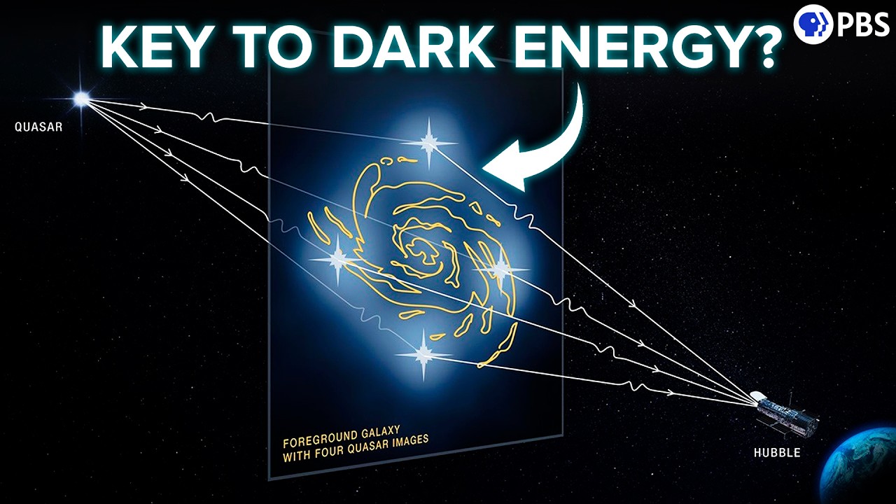
Added:Foundational principles of General Relativity, specifically how mass bends light to produce strong gravitational lensing, Einstein rings, and multiple images.
Understanding of parametric mass models in astrophysics, particularly the Singular Isothermal Sphere (SIS) and Singular Isothermal Ellipsoid (SIE) profiles.
Basic concepts of Bayesian statistics, Chi-squared minimization, and Markov Chain Monte Carlo (MCMC) sampling for parameter optimization.
Familiarity with observational astronomy data formats, coordinate systems (e.g., arcseconds, RA/Dec), and identifying lensed image systems.
Mapping the total mass distribution (including dark matter) of galaxy clusters using the optimized Lenstool best-fit models.
Reconstructing the intrinsic, unlensed morphology of high-redshift background source galaxies to study early galaxy evolution.
Applying time-delay cosmography to constrain cosmological parameters, such as the Hubble constant (H0), using lensed quasars or supernovae.
Comparing parametric modeling results from Lenstool with non-parametric (free-form) pixelated lensing reconstruction software like PixeLens or Glass.
498 views10likes1:45:36Original Release: 2020-01-31
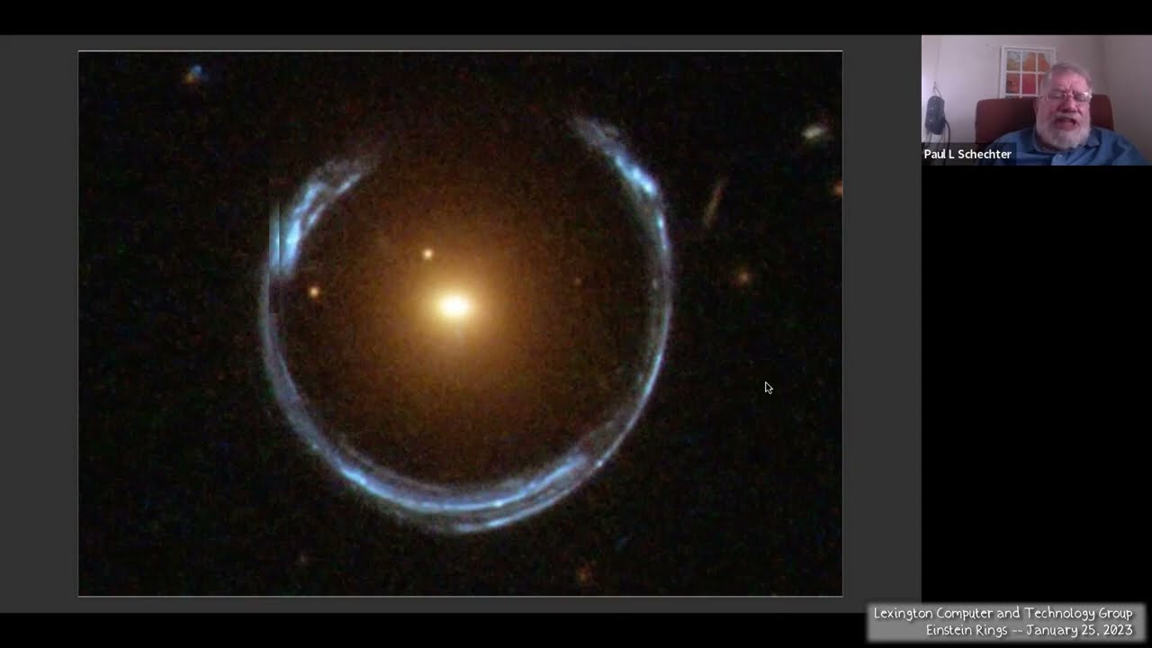
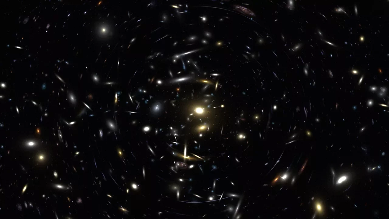
hi my name is michael hansen and in this video i would like to show you some solid practical examples on how to use lens tool or perhaps you could say a program like men's tour because this is what i'm about to show you here is sort of general in all cases for most of the software out there for modeling great seasonal NC so first of all i'd like to introduce to you the windows i've opened on my screen or behavior you see terminal where i'm going to type in commands you'll see that here I have a text editor at this point here you can see a list of different sources these markers here means that these sources here has been commented out and will be ignored file install and here you can see the model parameter file which I will also introduce later on so let's get started so the first thing to notice in this model that power file this is the primary parameter file for lens tool now this particular parameter file has been set up in a slightly different way because this parameter file I am actually not modeling or optimizing images giving optimizing a given per a set of parameters giving some images but here I'm actually doing the reversed I am giving minstrel some fixed parameters and then I'm going to put some images I just do this in order to show you sort of in a quite reasonable way how images will change when you change the position of the source so let me introduce the parameters for you here you have you can see it as profile and one one means that it is the singular isothermal ellipse if I for example Road 81 it would be the deep high profile so but here I'm going to use the singular isothermal ellipse the ik center and y sandrov's ax in oxygen with respect to this reference point up here I've chosen 64 dot for the red to sensation and - 24 for the declination you can actually use whatever what you want if you're modeling an actual cluster out there then ideally you would choose real coordinate systems which means that you would replace this with actual coordinates you derived from the images that you have from the Hubble Space Telescope where you have them now since this is the singular isothermal lips maybe I could write that here sorry you can see that I also have an ellipticity which i've set to zero here and i have an ankle petition which I have also said to zero because as you hopefully know if I have an ellipse I can always reduce the ellipse through circle by setting the ellipticity to zero or one depending on which system you're using and the angle position becomes irrelevant when we only have when we have a circle because if you rotate or circular around its center then no matter what angle you rotate it in it will retain the same sheep we also have did last the dispersion which I have said to an arbitrary number here which could be somewhat typical for galaxies 422 0.93 2 kilometers per second and the redshift also I've also chosen arbitrarily 0.3 96 some of you might remember that this is the exact same redshift that I've used in my master thesis then here down here we have to do ela or grit as it is called nombre means how large the grid can be for lens tool the standard maximum is 128 pelea means whether to use polar coordinates or not we don't use polar coordinates here and inland till is the number of lenses since I have only one s ie profile it's numbers 1 this source parameter here is sort of driven irrelevant because I have to shift in the sauce cannula observe binning I only been one so I get the full resolution you could set it to 2 or 3 or whatever you want seeing I have said this into 0.5 that is sort of excellent seeing on on where these two parameters is not relevant here they sort of just defines whether you take should put in some noise in the picture and how does not should be distributed in the sky determines how much background noise you would expect from the sky cosmology model one just means that we're using the standard cosmological model it's zero is the Hubble constant 70 kilometers per megaparsec second square I think it is Omega matter 0.3 Omega lambda Omega X 0.7 standard values and make a caves curvature it's zero there's no curvature and these are specifically defined in relation to the distribution of the dark energy then we have the Z line parameter down here where we can set some planes I have chosen to retain any but as you can see here if I put if I put in the phone here I would get critical lines and caustics for redshift this red shift this red shift this red shift and this red shift this is how large the grid should be in arc seconds so please remember that this parameter partyer means that it would be 150 times 150 times 2 because it is 150 on one side 150 on one side and 150 and 150 so it would be 300 times 300 the algorithm marching squares is the usual limit high and low defines how many much resolution you want on your political lines in the caustics if you choose to low resolution here then you would get holes in your krieger lines and the costings granted well i actually to be honest really don't know what this parameter part is is really about lynched who needs it but it is just a standard values champ some of you who know a little bit French might know that this means field so this means that my field for most of the outputs I get is 20 after it means it is 40 times 40 ounces all right let's go to the top you already know the reference parameter source it's my source list as you can see here mass means that I output a mass image pixel is where I get the images and verbals it just means that we get some extra information if I set it to zero you'll just get the absolute and necessary information to see that lens tool is running all right I'll just save it and then we can look on the saucepan here these two sorry these for a sources here is the sources I want to show you what happens when we move the source from the center and out the s sources here is some sources are already defined but I'll show you how it looked for optimization of a singular isothermal leads or sphere all right so let's start let's run lens tool with this parameter file here so let me just write install model dashing in sari then we can see that lens two runs and then we can try to open this file the image file that we got to make so here you can actually see and Einstein ring like I said the lens would be somewhere in here we can for example open a new frame and then we can open there in that fits here you see the lens and if we blink those you can see that hopefully see that the distance is almost the same from the lens now let's just go back to frame two so this is when the source as you can see here I've shown you the source is position at zero zero zero zero this refers to the ellipticity of the source and I'm using this is the position angle this is the wretched and this is the magnitude so this is not this disease that is the flux this isn't used in in England's tool but it is there all right so let's try to do some other things let's try to choose another source like this we still have no that's just wait a second let's use this again now we'll do what we do this all right sorry let's run the code again and you can see here that it performs best review transform and creating a scene filter and all sorts of things it's related to this you can see if I set the scale to set scale you can you can see some noise here this is the sky background that we can so it tries to emulate if we actually have a real image from a CCD definitely we'd get some noise both from the sky black background and from the CCD itself but I'll just set it to this value here all right so let's see what happened when I took move to source a little bit 0.5 2.50 now we've got two images you can you can possibly see I'll try to change the scale a bit you can perhaps see that they are little elongated even though this is truly a single eyes the thermosphere you can see that they are little in Anki but we don't have a ring anymore we have two images one here one here and if we blink again you can see that one image is fairly closer little bit closer to the lens than the other so I would surmise that the source would be somewhere around here which possibly is okay all right so let's go back to the images let's try to run it with where we've moved the sauce a little bit more of an little again and we don't see the images let's move they move some distance in this direction here but the distance between them is still the same but you can possibly see that this image here it's a little less magnified and this image here is also early this is the magnified and this is actually a little less magnified if I blink again you can see that the stores would be possibly somewhere around here and you can see that this image gets closer to the lens and this image gets further away take this set it to sink all right so let's move the source again this time up to 2.0 and 2.0 it fans to images as you can already see here let's take a look images that you see this image here kids little less magnified this gets deep magnified but these kids also little less magnified and if we blink again and see that this image is very close to the source now if we had the lens here remember that this is to the images if we had two lens you can probably imagine that we wouldn't see this image here because it would be obscured by the light from the lens please do remember that these images that I'm showing you here the image of the NASS here is a mass estimate from this run here so it doesn't have any physically to do with an actual galaxy but it's more to show you how the images and the source would be positioned with respect to the lens let's try to put another source in here because I must admit I was actually expecting this to be to be one image alone let's put it at four and see what happens now we get one image so let's take a look one image here and that is because the source had moved past the past the Einstein ring you saw the Einstein radius we saw the ring before so the source would be some probably somewhere around here let's put in lets blink it social be somewhere around here I think all right so let's try another thing I'm trying to make I'm standing again but this time we'll make it an ellipse instead of a sphere and you run again see what happens now you can see it says it it has found four images if we get a perfect Einstein ring it would probably say something like 50 images or anymore let's take a look see now with fine we've got something else we actually cut four images because even though we have an Einstein we have an singular isothermal sorry even though we have the source at the exact center of the lens we no longer have as an ass fear we have an ellipse and if we you can see if let's try to decrease the ellipticity and we would get something more like an Einstein you can see we still get four images let's try to see how it looks see now we're getting more like an Einstein ring that's a further decrease the ellipticity now we get nine images as you can see here and now we practically we almost practically got an Einstein ring you can possibly see that it's a little more thick around here than it is let's try to make it like something like this now you can see one of the nice things about lens tool is that you can experiment like this now we still doesn't see we have an image here in which an image now let's be fair and honest there are essentially virtually no completely spherical galaxies in the universe they are almost always elliptical in shape but they can be very spherical almost to the point where you would say that they are actually spherical now as you probably can imagine I've cheated a little bit because I'm also given the source a little ellipticity just a little but it is that all right so I'm going to show you an actual optimization I'm going to use these parameters I'm going to cut them so we have them always put them in a new document to make it as small as possible so that we can always remember these numbers because I'm going to close this part here I'm going to open another window but first I'd like to show you what we're going to Mars for so you can see we find two images here now remember like I said the singular isothermal sphere and also the singular isothermal ellipse doesn't provide us with the third central image somewhere in here it just doesn't because it is singular now if we choose deep high profile which is not singular or any other profile that is not singular we we get 30 which in here all right so let's take a look at the images now so these are the images that we're going to optimize for now what you would do in the sort of actual sense and no one what images are what here you can probably sort of imagine that these images belong to each other these images belong to each other and these images belong to each other and try to blink so you know possibly also imagine that for somebody we miss the source would be here for someone to be here and for us it would be yeah yeah but like I said what we will do in actual when you've got first of all when you got images of an actual galaxy with actual multiple images you wouldn't have images like this first of all you'll probably have a much better resolution especially if you use the Hubble Space Telescope but you would also we would also have images you would take in with you would take your observations your your images from your observations in different filters so all of these images here would have different colors so you could distinguish them but what you would do then you can use a program to find your images the position of the images find centroid but if you wanted to you could also let's reduce the scale a little bit so we can get a better understanding of where the centroids are so you can see here we would probably say that we have a centroid here somewhere around here so around here somewhere around here so around here and so around here nothing like that then what you would take your regions here take your regions this is one way to do it and change it to get it in coordinates like this then you would copy these coordinates here and put them in a catalogue which I'm about to show you now so here we have D optimization can lock I'm going to close these files here and I'm going to and [Music] the image file so you can see him delete these regions yeah and then delete this frame and delete this room make a new frame and then we're going to open another image that I have here here you have the images that I just shown you something like this yeah okay here you have the galaxy in the middle this is the lens and these are the multiples that you can see now if this works you will get to see where the image is actually it didn't unfortunately so we're going to do something like this sometimes happens like this you can see it again then we're going to just a scale so we can better see what's on the image yeah this is good then we're going to run the same command again and now you can see the images so 1 1 and 1 2 is here 2 1 and 2 tools here and 3 1 and 3 2 is here this is what you see here this is the position reference 0 means that design absolute world coordinate systems you could also take them as distance from a reference point in world coordinates then you would say 3 here step and then something 960 4 5 6 3 4 - 25 instead I chose something like that yeah - 24 but since it would screw up the calculations if I did it like this I'm just going to keep it the right way so let's look at how loops when we're going to optimize so the reference still the same then we have a mass part here still the same I've removed the source part here so I haven't got any sources of course because I'm giving Glen's tool images then I have an inverse part here it is how lends tool would like to invert the equation as you can see here 3 means that we're going to use it by easy and optimization 0.05 is the burning parameter if I set this to 1 I would get a relatively fast burning face in tryna try to run it Winston let's let it run you can see that the burning face went relatively fast but I might exclude some important parameter parts that stop it and set it to just check that let's try it again so you can see that the burning face goes relatively fast and then we're going to go into the sampling phase where we're going to assemble all different model render parts in order to find the best model now if I just stop lens tool and set the burning parameter to let's set it to 0.01 I try to set it to zero point zero seven one and see how long the burning phase takes you can see it explores much more of the parameter space you can see it here by the burning exploration here it takes a lot longer time to get to any true reasonable value as you can see this is usually not necessary a burning parameter value of 0.05 is usually enough to get a good burning face that's it mm instead let's go on the restart parameter file here the restart option here is not relevant what if I uncommented lens tool will create a restart file so my computer goes down or the server's restarting or something like that then I can just restart my calculation it's actually very nice because when you have a lot of multiple images and a lot of if you have a friction a very big cluster with a lot of multiple images and a lot of cluster members then the burning face particularly in the image plane optimization can be very slow take many days now here you see that in the other part I call this grill yeah will I could also call it grid which is more English I guess number still the same Pola still the same pelea and it's the same term in until still same I have one inline script means that I'm going to calculate the critical lines and the caustics for one lens because I have moment and then lens up that means how many I want to be optimized still one it is going to change in the other part I'm going to show you here we have the image file so I until means tool that I have a mold file you can see here one means that there's a file and this is the name mall WCS is not this is deep preheated deprecated sorry but I have it anyway form is how I want to optimize so if I write 0 let's do that I'm going to optimize in the sauce playing optimization let's try now see how fast it goes very fast as you can see but essentially like I said it is emphasized essentially it's wrong but a better word would be to say that it is emphasized this is table typically done like I said in the previous video to sort of narrow in your parameter space because I only have one potential here and a reasonable limited parameter space there's no need to to use the sauce plane optimization set M limit this part here parameter value here is set to 0 1 and 1 this should be 0 also this is basically means that if you have images in your image list like you have it here where you may have these are all emulated to be spectroscopically confirmed images that is we are reasonably sure that this is the actual redshift of these images if you have formatted redshift then these are usually very insecure and instead you can optimize for the redshift of the images so what you would write is for example 1 here because you're going to optimize this would be the name of the image so for images 1 1 1 2 you would write 1 like I've done for images 2 1 2 2 and so on you would use 2 and 3 you can also write specific images if you have that or list of images here but usually you write families of images this one here that you usually write means that these values here are strict and this is usually this is ignored when we are using the by issue and optimization sick post arcsec is the position error of the images in our sequence if you haven't Hubble Space Telescope image which with a resolution of 0.06 arcseconds you would usually use that for stannis but eventually you would crank up that precision mirror also in order to avoid including parts of the structure along the line of sight and such things in your analysis I'm going to show you how you can actually specify what signal position sorry what position error you should have so here's the mean sorry not the mean to meet of the parameter value the parameter file this is the potential for g1 I could also call it let's just call it cow and galaxy this is the parameters for this galaxy here now remember these images here are from a mock catalogue that I have created myself that is also why I know where the center of the images should be a sorry of the potential but the ellipticity should be the angle position the velocity dispersion and the redshift now the redshift is the same it has to be so let's just write it here 396 also check that I have done singing here Masius 396 that's very important again these are the initial values that I keep it I have been told that lens tool ignores this when you optimize I'm not sure about this but if you put them in anyway because they sort of give you an idea of where your potential is with respect to the parameter values profile is one because I'm using and singular lips I've initially set the ellipticity and the ankle position to zero because I'm emulating a circle now remember this is what we can test here I have actually set an ellipticity and an angled position when I created these images but we can try to first see how well singular isothermal sphere will constrain the parameters these actual parameter values and then we can try to optimize for the ellipticity here is the limit part i've called cluster 1 because I covered it that's called down also I have three free parameters here when we're dealing with a galaxy galaxy galaxy Lintin you usually dock these parameter values down because you're pretty sure that when you have galaxy galaxy lensing you only have galaxy galaxy Lanting so you can be pretty sure that the center of your galaxy is actually also the center of your mass but if you want to be absolutely sure you can also optimize for the center in y and x + y now as you can see here I have said X&Y center to zero point zero there's also another option I could set it to WCS then I would have to use you just change this then I would have to put in the center of the lens using these values you can see at the I can point with the mouse because then it would be go away but you can see here that if you look up in the top of these nine you can see there's if Kyle fk5 then you can see there's an alpha and a delta and these are the world coordinate system coordinates of this galaxy so I would put that in there and step I don't want to do that because it is not necessary so when it's written like this it means that this is the distance from the reference point in our seconds and this is the same here I'm going to explore from now this is very important when you do this minus 10 and 10 means that it's going from minus 10 to 10 so it is minus 10 grid respect to the reference point to 10 with respect to the reference point so if I for example imagine that I had another guy Anka see here I couldn't just use minus 10 and 10 instead because this would be a completely different position with respect to the reference point so I had to use that all right and I'm also only optimizing now for the velocity dispersion as with the single isothermal sphere which I just opened up so I'm going from 10 to 700 because I don't have many images and I don't have I don't have many feel free parameters so it won't take that long to optimize even though it's going to take a little while let's try to run it as it is I'm going to save it let's try to see what happens remember that I'm optimizing in image plane mode now so it will take a long time so what happens here is that as the burning face here the Berman's burning values here approaches one we say that the burning has converged and then we started when the burning face has converged with it which it has now then we start the sampling instead now for some reason my computer doesn't like this is the little laptop doesn't like to be run as hard as it is here now I might get a little bit of result by letting it use another processor let's use true now you might ask yourself why don't I just use all four processes on my computer I have this is a call by five so I have two processes and two additional threats from hyper-threading but thing is that when you are dealing with a relatively low number of constraints and relatively low number of free parameters especially the constraints by letting the computer use or your server use a lot of processes you would actually use more processing time on switching the calculations between all the different processes then you would do in the actual optimization since I don't expect it it's very interesting for you to see these numbers slowly climb up I'm going to pause the video and then return what it is when it is done see you in a bit all right so now you can see the run that's finished you can see the chi-square you can see the evidence and you can see that it has calculated create the lines and caustics for these red shifts here and you can also see that we have a mass fits file now you can do a lot of things with these outputs here I'm going to show this results from a few of them so let's first look at the chi-square it's 38 let's open the best top part so you can see that we have three three parameters three to get degrees of freedom and we have a chi-square of 38 and we as you saw before we have a position error of 0.3 now I'm going to show you a way how to deal with this because the ideal case is to have the number of degrees of freedom should be the same as your chi-square number so you can probably imagine if I set this to be to be lower like 0.01 I would get a higher chi-square alright so let's try to calculate this I'm going to use ipython calculated we're introduced Thailand extension like this pilot detection extension alright so the idea is to take when it starts up the square root of the richest sorry does not the redshift a chi-square thirty eight point four three six form divide it by the number the degrees of freedom that's three and then multiply that by zero point three zero then we get one point O seven let's put them in yes let's run lens to look in while the install is running I'm going to show you something else you might have noticed that I used a command called purely this is a standard command that comes with Linz tool so you if you have lens tool installed on your system then you also have the Paley with this you can take any file that you might have containing coordinate points or position points for images that you have the potentials that you have calculated the position of the cluster members if you have some of them anything you can imagine that lens tool can read you can output this directly to ds9 as I have here and you probably noticed that I used a command where I wrote purely and then the image WCS file then I wrote red because I want a red color I wrote zero zero it refers to with a pillar should automatically clear any image some any new region files that you might have essentially it's the same as saying delete all regions and then I used point last because I want a point like this if I don't use point I get a circle with the same radius as you seen here so it would be a radius of 1 R seconds no ellipse so just be circle but here you can see and this if you have a lot of images that you have put in for example from an article you want to be sure that you are actually having the correct position of these images and you have a lot of images then using the very command and then shaking all these images is a very good idea alright so this is one way to ensure that you are actually giving lens to the right the right images I'm going to pause the video again and then we'll the Tran went down to my session is almost finished see you later so now that Lynch tool is almost finished let's take a look and see what the results might be alright it's finished so let's take a look at the best of pass on this gives us the best parameter value so we have three degrees of freedom still we have a kind square of three so in this essence we have one when we divide the degrees of freedom with our chi-square we get one which is what we wanted so let's initially take a look at the parameter values so we gone minus zero point two seven as the center zero point two one it's fairly close we got four hundred and three after the last two dispersion but the reason reason why I did this is to get correct errors so let's try to use another tool that is also included we'll instrument called bias results that peel it's a Perl script so what this tool will do is to read the bias that that file you can see that we have six columns here 20,000 lines because there are 2,000 different models remember that lens tool for some reason adds one so if I written 2,000 here I would get 2010 lines 2001 model but I want 2000 just two because that's why I am you can see here the arrows so we have the position X the best value is zero point two seven three two that's what we got here right yes three two but the error is if you look at the Gaussian here it is plus minus 0.3 so somewhere around zero and to me but you can also do that this arrow here it is somewhere between almost plus one minus one so the best parameter value that we get is definitely within zero point zero which is what we gave the model and the same goes for the Y zero point two months three four theaters is plus nine almost plus one and minus one point two one so again within zero point zero now remember we are not actually modeling in this system in the strictly correct correctly because I have used an ellipse this is an singular isothermal he lives that I am trying to emulate or sort of estimate by using a single isothermal sphere so in essence you can sort of check how well the singular isothermal sphere will do for a clearly elliptical system let's look at the velocity dispersion for the best value we got four hundred and three point three of just four hundred and three and we got plus minus thirty eight sorry we've got plus thirty eight minus thirty seven so definitely the correct value is within our air Abbas you might also notice that the median is close above the median and the mode is closer so the median you hopefully know it is the median the mode is the most prevalent number so this is the number that is found in our biased at that file the most times so let me just open the box that death so you can see it mr. so you can see we have the number of samples we have the likelihood we have the position of x and y of 1 and the velocity dispersion and then we have the chi-square and you so have you can see that we have ten lines here with 1 10 9 0 to 10 9 3 and so on because that tint changed for each of the models here now all of these lines here all of them represent one particular model that linsell has created and remember attested sorry and remember the lens tool tested in this case 20000 it's 2000 different models so there's a lot of them and then this tool here biostat that uses all of these numbers here to calculate these values here so what what is that for well as you you might look at the best up our file here and well if you are working on a system that you don't know what true values are you wouldn't do what I'm suggesting here but in this case here where I actually know what the corrector lives I used to create these images with ha I could look at these numbers here and say oh it's 422 430 that's not close really and even this is off it should be much less but when I look at the error bars you know which I calculate from the biased of that particular the asymmetrical errors here at Sarris is wrong over but it said ninety-nine point seven percent confidence interval or three sigma confidence interval actually see that my numbers are to some extent fairly reasonable within dear Abbas even when I'm trying to approximate an elliptical galaxy with a spherical mass model mass distribution but let's try to run it as it is so I'm going to add two new three parameters in here I don't you add the ellipticity which I'm going to say well I'm going to steal points in run to 0.99 so I'm going to explore all the possible electricity's I wonder to some extent a good now this is not the the precision on the parameter value or the parameter space exploration but it's how many precision numbers I want on my output alright and let's take the other is the angle position so I'm going to write in to us I'm going from 0 to 0-2 I just wonder I don't need the precision to that higher to be that high on the angle position I'm going to reduce the signal position and the arrow 200 points just put it at 0.5 it will make the optimization a little bit faster and that's run rinsed those two again remember now I'm actually recognizing that I might have an elliptical system so I'm using the singular isothermal leaves as it is now you can see that I have five free parameters and I have six constraints now you might now imagine what if I only had to multiple images and wanted to use this singular isothermal flips well you're correcting assuming that I might have a problem with that but as I said before when we have galaxies galaxies lensing we are almost always sure we can almost always assume if not always that the mass center of this galaxy is at the center of the emission of light so in that sense I can remove two three parameters but I still have three so what could you also do well you might try to do spectroscopy on your galaxy and then figure out what the velocity dispersion might be and when you know the velocity dispersion you could remove them as a free parameter you could also remove that as a free parameter and then you have from two images you would have two constraints and you would have two free parameters so that work but you are correct in assuming that given only two images to multiple images and a galaxy and one of wanting to emulate this or optimize this is an ellipse you would have a problem particularly because in real galaxy situation you almost always have some kind of external sphere so in essence you have the galaxy creating these images that you see but you usually also have galaxies around this galaxy or something else chirping the field here a bit so they will move the galaxies a bit around so you would almost always have to include some kind of external shear when you are in optimizing galaxies galaxy lensing and that would include at least two new parameters for this external shear so yes you need enough multiple images in order to optimize such a system successfully we're going to pause the video again and then return when the optimization is done alright wildlings tool is still running I have to ship back and forth between the position error in order to get closer to one and now I'm down to 0.03 so let's see what gets there but before I'm going to show you that I want to discuss with you or show you something else now as you might have seen I have six number of constraints and some of you might have also seen that I have six images so you might be led to believe that when I have six images I have six constraints but that is not the case the number of constraints that you have in a given system goes as the sum of two times n minus 1 where n is the number of images in a particular system so in this case I actually have 2 times 2 minus 1 plus 2 times 2 minus 1 plus 2 times - Lance one that gives me six but I'm going to show you in a bit just a bit that when you have more systems with more multiple images you don't only have second the numbers constraints that are equal to the number images that you have so let's take a look if it's finished it is so now I have an error of 0.1 - now I don't think I'll get it any better than that let's do that it best on Python yeah I think that's reasonable now it should be closer to 1 but it's ok it's hard to get it to 1 because well yeah it is so let's look at the numbers now we can take a look here and now we can see that it is actually quite reasonable so we have X sin x minus 0.02 that is almost zero the Y centers through point zero seven almost zero the ellipticity is 0.4 the true position is 0.303 the angle position is 126 the true position is 123 the velocity dispersion is 104 23 the troopers velocity dispersion is 422 so let's look at the arrows on our system so we get an error of the X in plus 0.04 5 in both cases for the Y we get plus OH point 9 and 0.9 I'm looking at these asymmetry carousel here for the ellipticity we got 0.4 and the Euro bus we get plus OH point 0 3 and minus Oh point 0 2 so that is fairly close to the true number that the angel position we get one hundred and twenty six point one if you will we got plus two point 1 and minus two point five that is also means that our angle position is reasonably close to its rightful position and of course the velocity dispersion is as close as it can be 423 and we got minus 2 and plus 2 so within the error bus we actually got a quite good representation using this system here now of course as you know I you can probably see here that I set it down to 10,000 lines and Stefan are set it down 2,000 answer a thousand different models instead of 2,000 different models that might be the reason why we are close but we could probably get closer by using 2,000 stand but nevertheless given the way that we are optimizing these things remember that we are choosing the most probable model from a large set of different models our parameter values actually got pretty close and all of them within the Erebus fits the actual values all right I'm going to close this and next I'm going to show you what we can do with a more complex system so let's just change the values that we have and change this here so here you see the mass distribution from again I created a mock catalog and this time we have a bright cluster galaxies here in in here together with the center of the cluster almost spherical cluster profile it has a small electricity and then we have some cluster members placed almost you can see that they're placed symmetrically but I've just put them there and then I have also put in some sources at a vast number of different redshift so I'm going to show you the first a list of images that is reflected the list of sources so let's take a look at yeah sorry let's see yes let's open de marmol sir yes so you can see here here we have a vast number of images let's take a look at the images you can see them here cedar arcs you can see that when we're dealing with a cluster we get much more complicated system now of course I've added more sources but nevertheless we also have many more images we actually have 28 different images from 8 different sources so now we can take a look at the idea we had before about the calculations so let's see what we got 2 times 3 minus 1 plus 2 times 3 minus 1 that is I'm going to 4 here that is plus 2 times 3 minus 1 plus 2 times 3 3 much 1 plus and we have the 6 and it's also 2 times 3 minus 1 just might go wrong because it's a lot more complicated so here we have 5 2 times 5 minus 1 plus 2 times 3 minus 1 that is 2 5 here and the 8 also have 5 images that is plus 2 times 5 minus 1 it should give somewhere around 40 constraints now you can see that we have 28 different images but get 40 constraints so that is partly because we have some of the systems we have up to five images instead of the usual two images in the system before and you can see that I didn't have three images now you might remember the idea with critical lines and caustics so for the images the sources that gives three images we can conclude that the source is within the outer caustic for this particular redshift and the images that the sources that gives five images are within the inner caustic for that particular redshift you can also see that we have a much more variety much larger riding on the redshift will give us from one point one five to five point four all right so let's look at the model parameters now as you can see here I have included parameter values for deep I profile for cluster halo as you can see here I've set the core radius to 90 the cut radius to ten thousand should be a large number the ellipticity is 0.3 so it's not that much elliptical it's a little offset compared with cluster galaxies that's also that catalog it's called cows but you know so we can see a ten list of reference galaxies it is positioned you might not want you might not be able to extract that from here but you can see our reference point is 64 and minus 20 and here you have sixty three point nine nine nine six four nine that is almost 64 and there you have minus 20.000 to 4/7 that is almost minus 20 so this is in this macro center hour cluster helos a little offset not much but it's a little offset you can also see that the velocity dispersion is twelve hundred and fifty for all the cluster members the core radius has been said to 0.5 teen kiloparsecs the magnitude is from the brightest it is 17 the Sigma the velocity dispersion has been set to 375 the cut radius has been set to 60 and the slopes has been fixed to four and two point eight five seven one as is consistent with constant mass-to-light ratio All Right see ya that is okay all right so let's try to run this you can see we have 40 let's try two we have calculated that we have 40 constraint let's calculate the number three parameters so we have one two three four six here and we have two here so that's eight free parameters and forty constraints so we are reasonable winning the limits of being able to constrain this system alright so well let's run it before I run it I should be I should tell you that on my laptop I'm going to run it in their sauce plane optimization mode I use a position error of 0.5 I have said fairly open parameter priors as you can see here - 10 - 10 in the position 0.01 to 0.99 in the ellipticity and so on the idea is that I first run this particular model here in sauce plane and then I use that to constrain or retain restraint my priors to run it in image plane because given that I have added many more multiple images and also most systems remember that even though I have only 8 free parameters I have something 11 galaxies within the system so I actually have 12 different profiles in an actual sense even though the 11 of them is optimized biased scaling relations and not individually like this but let's run it and see what happens so you can see even in source plane optimization in sauce plane optimization even using the many more free parameters and the more constraints it is fast it is reasonable fast but still takes a fair amount of time you can probably see here that even though the burning face perhaps I should probably try to change something before I just don't change that save it to all four and try to run it again see if that helps all right just like before I'm going to pause the video and then come back when this run pass almost concluded see you in a bit all right so the run has concluded in the sauce plane on to my station I've all been the best apart file remember this is still sore spleen optimization so as you can see the X Center the Y Center somewhat off actually a bit the ellipticity is reasonably close the angled position is also reasonably close the core radius in kiloparsecs it is somewhat off actually a bit off the Padres is not optimized so it is the same and the velocity dispersion is also to a reasonable degree fairly close even though given that I am using soft plane optimization so let's take a look at that it is so that since I chose the magnitude the reference magnet you to be 70 17 sorry this galaxy here with the magnitude of 17 is going to represent the reference numbers so you can see that the cut radius has been said to has been found to be 414 where the reference is 375 someone off and the velocity dispersion is 297 whereas sorry the cut radius in oxygen is 93 while the true no sorry the cartridge has been set to 60 in kilo Pathak's whereas the cut' radius found in lins - lins sauce playing up to my saying optimization is 414 so that is highly off 7 and also that the lastly dispersion was a - 375 whereas what was found was 297 so this is also read to a reasonable degree fairly off that's just that I said the correct values I said for this is okay and 2.85 71 this is also okay so this is most likely because I am dealing with sauce plane optimization so let's run the biased up advice for salt and and see what we got well you can see that our cadres is somewhere off you can see here that we have a red number this red number means that for some reason our cut radius for the galaxy's has hit a limit so one of these numbers and I'm going to look at the mode is close to the limit and let's look at what we got because we said it true now the thing is that we set the card radius between 110 and 104 some reason this is offset so another little trick that you can use is to go up at the output from lens tool you can see here that we have four point three eight here four point four three eight this says that at redshift 0.31 arcseconds is equal to four point four three eight and down here I got the cut radius here in arc seconds so I can use this command here and then set scale equal to this number and then I get it in what you call it in in kilo Pathak's now you can see the node is four hundred and twenty eight and I have limited add I'm sorry I'm just going to run it again like this you can see it it's 96 Dawkins oxygens I have said to cut radius to 100 so I could probably set it to something like 150 and then run it again and so I could go on until all my numbers are no longer red when I have done this a couple of times I will go over to reduce the price conceded values here to more constrain them more at the actual values and then run the model again but this time optimizing it in in Seoul in huge playing optimization now I'm going to do that on a server and as you'll probably notice when they started it will take a reasonable longer time to converge even for a burnin face so I'm going to let you see that I started and then I'm going to show you the result when it is finished it will most likely be somewhere around tomorrow so even with a highly reduced number of cluster members I have only 11 in my max model there were 175 I have 40 constraints from 20 images somewhere around 20 images in my max model I only had 10 images alright so let's start it now as you can see I still have 40 constraints and 8 free parameters which is good but as you can probably also see the optimization quickly slows down in image plane optimization so I'm going to pause the video for now and then return when the optimization is finished all right so now the model the cluster model as I have called it up here has finished and you can see now that I have actually run the biased results peel script again and now you can see that I have no red results meaning that none of the parameter outputs that I get I have gotten in the past that that farm has hit the limit with my price but as you can see some of the grammar values are still highly offset compared with the true values all right one other thing that I wanted to show you now before I showed you a way to calculate where you got this title here the chi-square and then I use the model file and then I change the signal position error and then I ran it again now you can also use another file called best up top path and then you can change the chi-square the difference is that the best model this table uses a Gaussian prior value meaning that these priors actually trying to stay fairly close to the primes that you give it because you are here assuming that you have the best model parameters that you can get so I'm going to run this model it should go fairly quickly but nevertheless I'm going to pause the video and then return with it has been it has finished all right now the model has run through and I've calculated the position error I'm going to copy that number into not the best that power not the model but path but the best up laptop this file will still optimize the model but it should retain the values the optimal values that it gave me and instead just reduce the chi-square all right as you can see here I have refined it a bit I got it to 1.07 almost won I refined my position error here you can see Oh point zero six eight now as you might remember when we ran this model only as a singular isothermal sphere we got away with almost 1 in our state in our position error here we can go as low as 0.06 and get a reasonable chi-square now I'm going to be really extreme I'm going to let this one all the way on to 20,000 different models that's 200,000 inputs in the past at that and then I'm going to talk with you again when the optimization has run see you in a little bit so I'd like to show you now the results from the run of the single singular isothermal sphere with 200,000 lines in the bias that biased at that file or 20,000 different models so the run has completed and let's take a look at the biased of that file so as you can see here now the perl script takes a lot longer time to calculate the results because before it only had to look through thousand 2000 lines now it has to look through sorry i'm 20,000 now it has to look through 200,000 lines but let's compare the results again you can see we have the the best result here for the X and the y as you can see here zero minus zero point zero two eight six with an era of plus zero point zero five five eight minus and minus zero point zero six two one is as close as it can get to zero point zero and likewise you can see with the Y position here at the center of the y position zero point zero save one five with an error of plus it's a little higher theorem here but again it is very close to zero point zero the ellipticity as you can see here zero point nine three nine six and i chosed three eight three but again the error is plus zero point zero five three and zero point zero four five so again it is reasonably close position angle 120 five point five and I chose 123 point eight nine and again with the arrow box you can see it is as close as it can get and finally the velocity dispersion 421 point seven I chose phone in twenty two point nine so again reasonably close as you can see next I'll look at the results from the the cluster simulation that I did so I finally managed to get the last model we looked at running and now able to show you the results alright so as you can see I had to fiddle a bit around with it as you can see here and take degree of freedom and still the degrees of freedom is still 32 but I Chi square got to 30 so we can just simply calculate that 32 32 divided by thirty point six one one teen it's almost one so it's actually fairly okay and if you look at the best up file you can see that I got precision arrow down to zero point zero six nine zero point zero statement which is also pretty okay usually when dealing with sorry true systems not mob systems like this you'll get a much higher and pushy shanira let's took a particular look at the results the original results that I gave the model was 0.15 our best result is zero point zero nine nine zero point one sort of and the Y Center was zero point twenty and we got 0.23 which is pretty close our ellipticity why we created these images from these images here was point thirty and we got point thirty the angle position was 120 we got 119 point eight which is almost 120 the core radius we set it to 90 and kiloparsecs remember that this is in arc seconds so when we convert it the cone radius the model gave us was 92 and of course the pod radius was fixed our loss to dispersion for the cluster healer was 1250 we got twelve hundred and forty nine point four this is pretty damn close I'll say let's took it take a look at the cluster members as you can see all of these most of these parameter values here are fixed this is because this is the reference galaxy we can just look at it because it will give us the correct results so as you can see here we gave it Cod radius of 60 kilo past six whereas the model cave was 76 so it's almost seventy seven is a bit off not much but a bit but in respect when we look at the velocity dispersion signal value we gave it 375 and it gave us 375 Smeg on so one explanation for this for this is that like I have said in the previous video with the results from my master thesis presentation you actually need multiple images around galaxies in order to constrain der in order to constrain these values here through a significant degree now if we look at over here I have the results with Erebus do mind you that I increased the number of samplings to 5000 so we got 55,000 lines instead of instead of the usual 10,000 lines but as you can see here to look at the x position of the halo that was a little off it was 0.09 96 but we got 0.07 so let's try to put that in 0.096 plus zero point zero seven where was it seven one six in one we got zero points 17 and the correct number was 0.15 so we actually within 99% certainty with with the correct value remember again this is the best value we got here and also what was also a little bit off it was it was this number here the best value that we got was 17 point let's put that in 17 points remember this is in our seconds right so same in between point 23 76 and then we need to take minus one point one eight four six it gave us 16 point zero five three and I don't have the correct number in in in our seconds so we need to convert it and I think I have to correct method in here somewhere that was I'm gonna take a little look and then I come back to you all right so now I'm ready let's take the virus results then we can put in another parameter by putting the scale this number here means that 1/2 second which is the values that we got here for most of them is consistent of is the same as 4 point 4 5 4 kilo past 6 in that particular redshift and that cosmology so let's try to run it now you can see the depreciation angle changes and that means that if we compare these values here they will be highly off 101 119 and 209 so we can't really this is not something we should look at but we can see here that we get the cut radius let's take a look again we got 76 yes and then we can subtract 5 so how quick eyes will tell us that this is not enough simply 6 plus 7 7 6 3 minus 5 4 7 0 it will give us 71 it is still 11 off but again please remind yourself that we don't have multiple images around all the cluster members so that is probably most likely why this is this value here is somewhat offset all right another thing I would like to remind you of is that this is exactly what I meant by having a system where the lensing equation when we invert it this is what we have done here we've inverted the lens equation is nonlinear if we had a linear system if this were a linear equation then giving giving giving lends tools on masses in here can open them I think I have that here they are if I can give links to all these masses here put in some sources and then get these images here giving some parameter values again remind you that I am talking about a linear system if I then invert this system so I take these images and then try some parameter values and try to find compare to the best fitting with the images then I would get in a linear system the exact same numbers completely exactly the same numbers this is constitutes what is meant by a linear system so for example if you take let's say if you take your distance you have traveled and divided by then let's take a simple example I can calculate it here so let's say that we have this is a linear system you all know that if we take the meter per second then we did this is a velocity right so let's say we have traveled a thousand meters and it took 250 seconds then we know we are traveled with 4 meters per second so if we invert invert the system so let's say if you travel with 4 meters per second for 250 seconds we will travel a thousand meters so this is a this is an example of a non linear system the linear equation you can see it might not be that obvious to you here but I have actually inverted the system first I took up here I took the meters that I traveled and divided it by the time I traveled and then I got a velocity in meters per second then I inverted this equation here so instead I said well I'm traveling with meters per second and I travel for 250 seconds how many meters to add travel if this were a nonlinear system I might as well have gotten 560 meters of course these calculations Hanlan's tool are much more complicated complicated but the idea is still the same so given that this is a nonlinear system and of course this is a relatively simple system I could have put in now I put in 11 cluster members right and usually used somewhere between 40 and almost 200 cluster members we also in the new data from the muse telescope unveiled a new muse instrument on wheels he we got over 200 multiple images for the cluster I've analyzed in my master thesis I hope that you I hope that you had gun a little insight into a how lens tool actually works of course I have used market catalogs here but the principle idea in optimizing a system in linz tool is the same I'll just quickly recap you get some multiple images then of course in a true system you would take spectroscopy of all these images that you can see on all of them that you can get spectroscopy off because this is a a mock catalog without trellis you cannot really distinguish the images from each other you will be able to do that in a true system in real system because you can also see where the galaxies are positioned is likely that we have a galaxy here let's try to blink [Music] yes you can see we have a galaxy here that influence these images here and also the same down here right so galaxies multiple galaxies or the cluster members will only usually picture the images but the central part galaxies in here might possibly create multiple images as well but the idea is to recap that you set up your parameter file with your potentials that you want to optimize for this is the priors that you put in so this is sort of the way you restrict you our exploration of the parameter space and down here you could have you said if you have if you have cluster members instead you could also put all the cluster members in like a potential like this but let's say you have a hundred cluster members and you have six free parameters for all of them let's say that you exclude the center's so you only have four then you would get four hundred free parameters just for fun custom members alone so that that's not doable instead you include them in this potential file here where you include the position if you want to include the shape of the galaxy it's here so you get an electricity from an A and a B the minor and major axis major and minor axis and then a position angle here then you include the sorry then you include the magnitude here and the luminosity of flux here is not used remember that whether you use a B or any other kind of magnitude system is practically irrelevant the only only the only important thing is that the magnitude that you put in here system that you use here and the magnitude that you give it here isn't the same system so you can say if you use the brightest galaxy as your reference galaxy you'll almost always get the same magnitude here then again you set in priors and in these prize you can sort of use the price that you would expect usual galaxies to have so I would say cut radius between 10 and 150 arc seconds is probably okay and again a velocity dispersion between 10 and 600 is also okay for galaxies usually you could wrap oh you could you could actually expect this to be between 100 and 60 but here you include the possibility of very very faint small galaxies then you put in some other parameter values here in lens tool that I have already described you set the inversion parameters how much you would like to how much detail you want to get from the burning face you set here somewhere between 0.1 and 0.05 is usually consistent for a very detailed look and then you set the how many assembling you want to run in order to sample your parameter space again it's very simple if you set a low number of samplings you are - my saving is relatively fast but you might exclude the best parameter value set if you set a higher number of samplings for example twenty thousand I selected then you would most likely hit the best assembling point but it would take a much longer time to sample especially if you have a large cluster and then you said in here in the image file where you put in your images Moll WCS you can exclude because this is deprecated but in the former optimisation here you select with zero you're running soft pain optimization if you set it to minus one you'll run image plane optimization you have to include this value this parameter option here even though you are not optimizing any multiple images for some reason lynched who needs this parameter value here in order to run and finally the position mirror you select something that seems reasonable if you lose you're using Hubble space in between you can set it to the pixel resolution so usually that is either zero point zero six five or zero point zero three but most probably on real system you would end up the position error somewhere between 0.3 and 1.3 something like that alright that should be all of course you have if you have any questions you are welcome to put some comments on this video I hope you have enjoyed it and I hope that you have gained insight into the basics of how lens to words thank you for watching
Up Next

10:16
Understanding Development: Concepts, Theories, and Dimensions
@ImranHossainBhuiyan
161K views•2019-03-15

12:54
Triumph of Orthodoxy Icon: Byzantine Art & History Explained
@BenCallan
2.1K views•2024-08-06

9:49
FastAPI vs Flask vs Django: Choosing the Right Python Web Framework
@TechWithTim
302.5K views•2024-05-26

1:42
Game of Thrones Opening Credits: A Cinematic Analysis
@gameofthrones
46.3M views•2011-04-18
Related Study Plans & Knowledge Roadmaps
Structured learning paths in General & Interdisciplinary Studies
general-studies
Elevator Engineering: History, Physics & Cities
01From Hoists to Safety Brakes: The Dawn of Vertical Lift
02Hydraulic vs. Traction: The Engineering Physics of Elevators
03Modern Speed, Safety, and Algorithms
+ 2 more learning modules
12h5 modules
Explore Roadmap
general-studies
Rubber: Material Science, History & Geopolitics
01Origins of Natural Rubber & Mesoamerican History
02The Chemistry of Natural Rubber & Vulcanization
03The Geopolitics of the Rubber Boom & Colonization
+ 2 more learning modules
12h5 modules
Explore Roadmap
general-studies
Containerization: Evolution, Logistics & Trade
01Ancient Trade & Bulk Cargo: Amphorae to Barrels
02The Industrial Revolution & Cardboard Packaging
03The Containerization Revolution: Malcom McLean
+ 2 more learning modules
12h5 modules
Explore Roadmap
general-studies
Textile Tech: Evolution, Labor & Global Impact
01Pre-Industrial Textiles: Handloom & Cottage Industry
02Mechanization: The Spinning Jenny to the Power Loom
03The Factory System & Global Labor Transformation
+ 2 more learning modules
10h5 modules
Explore Roadmap