





![[UT#1] Comprendre les sommes de Riemann (L'idée)](https://i.ytimg.com/vi/R6ge0QBu3Nk/maxresdefault.jpg)
![G12S Calculus Chapter 5.2 + 5.3 [ALL GRIDS]](https://i.ytimg.com/vi/qryTBzuZmTg/maxresdefault.jpg)
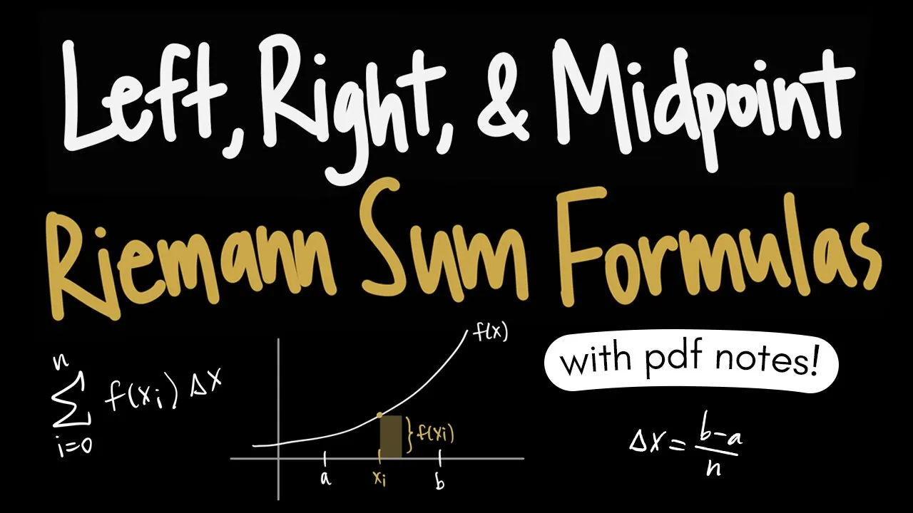

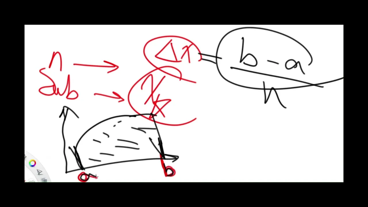


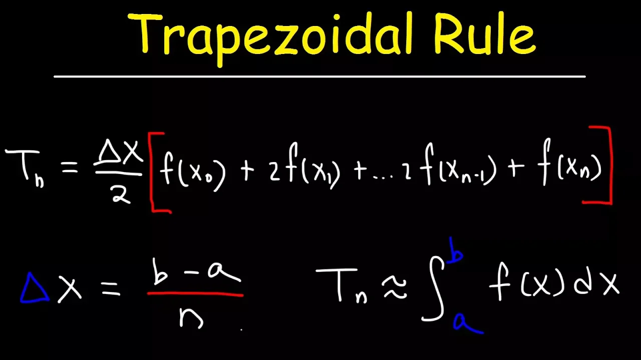
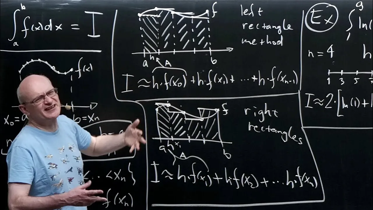


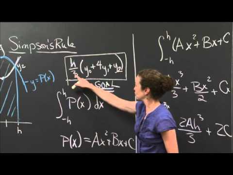



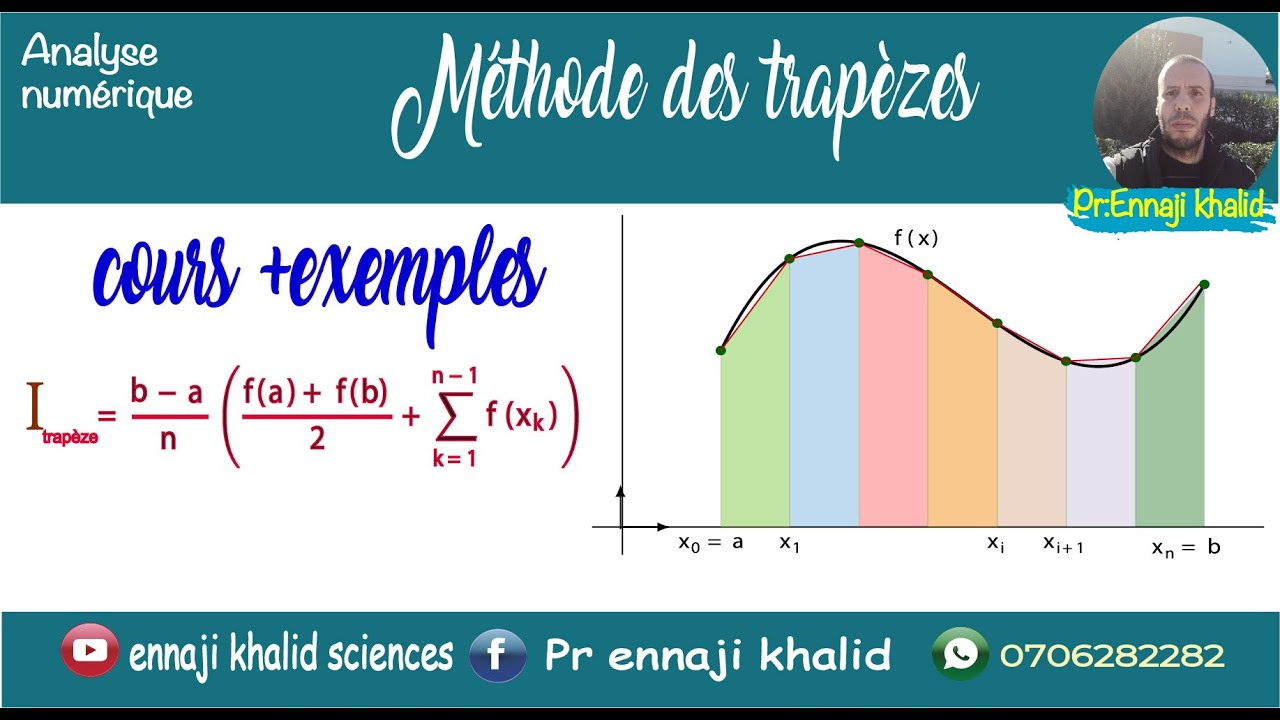







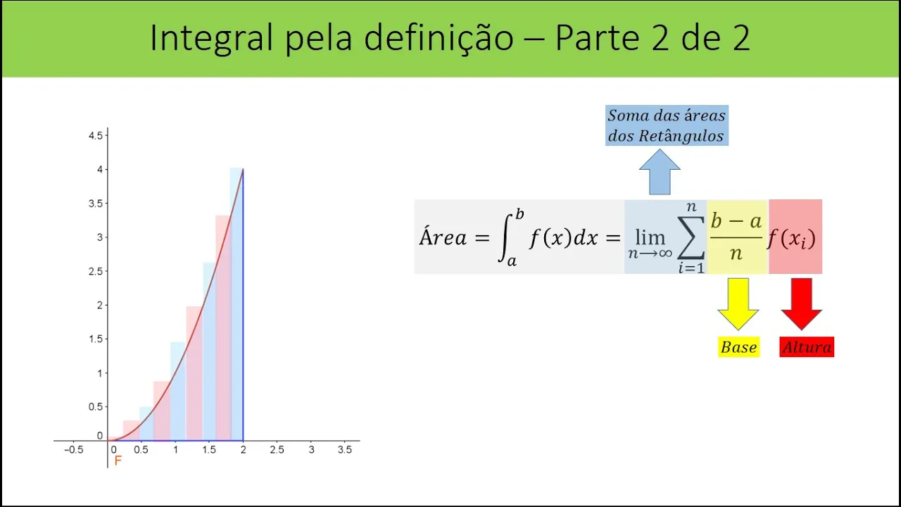
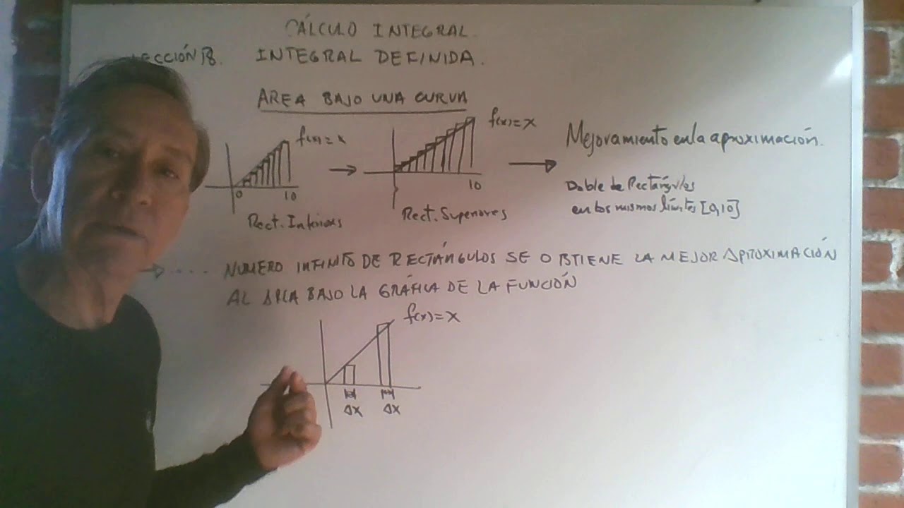
The trapezoid rule approximates the definite integral of a function by dividing the interval [a, b] into n subintervals, calculating the width Δx = (b-a)/n, and then applying the formula: (Δx/2) × [f(x₀) + 2f(x₁) + 2f(x₂) + ... + 2f(xₙ₋₁) + f(xₙ)], where the first and last function values are multiplied by 1 and all intermediate values are multiplied by 2; this method uses trapezoids instead of rectangles to estimate the area under the curve, providing a more accurate approximation than simple rectangular methods.
Trapezoid Rule Explained: Approximating Definite Integrals
Added:The concept of a definite integral and how it represents the accumulated area under a curve.
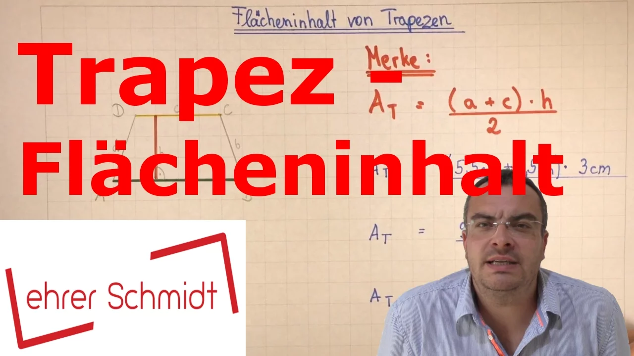
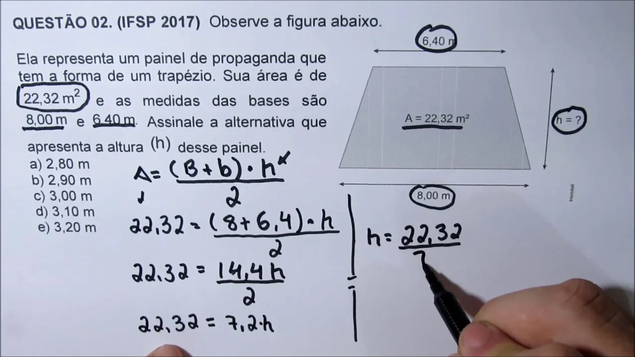
The geometric formula for calculating the area of a trapezoid.
The fundamentals of Riemann Sums (Left, Right, and Midpoint) as a foundation for approximating integrals.
How to partition an interval [a, b] into subintervals of equal width (delta x) and evaluate functions at specific grid points.
Simpson's Rule, which uses quadratic approximations (parabolas) instead of linear ones to achieve higher accuracy.
Error bound analysis for numerical integration to determine the maximum possible error of the Trapezoidal approximation using the second derivative.
Implementing the Trapezoidal Rule programmatically using software or programming languages like Python (e.g., NumPy/SciPy) or MATLAB.
Adaptive quadrature methods, which adjust the step size dynamically depending on the behavior of the function.
661.2K views3.7Klikes7:22Original Release: 2009-02-23
okay in this video I'm going to do examp an example using the trapezoidal rule um and all this does is you're approximating the area underneath a curve using trapezoids um sometimes you'll use rectangles um just another way to do it is to use trapezoids um without doing a lot of justification basically the formula is this it says you can approximate an integral from A to B um some function it says basically what you do um assuming we chop it up into n Pieces okay it says we take Delta X over 2 which is just the length of the interval divided by the number of pieces um and then it says we just take the function evaluated at the first point plus two times the function evaluated at this next one um notice the twos all inside of here until the very last Point notice that doesn't have a two on it um again where X ofi is given by this formula A+ I Delta X obviously this is probably not the place you want to start if um you know you're just now looking at integration um but if you've seen the video about uh that I did about um understanding the definite integral um I think this xabi and this Delta X notation should be familiar so I'm going to make mine relatively straightforward just to hopefully make the numbers work out a little bit better so it says we want to approximate the integral from 1 to five of 1 plus x^2 and I'm going to use four trapezoids if you were to graph 1 + x^2 so I'm just going to draw a little picture here 1 + x^2 would be um a parabola shifted up one unit from x = 1 to xal 5 and it says we're going to chop this up into n Pieces okay so Delta X is going to have value B minus a so that's the right Point minus the left end point Point divided by the number of rectangles so we'll get 4 over 4 or 1 so that's the width of each one of our intervals again we've chopped our interval from 1 to five up into 1 2 3 four pieces each one has width one so you can see that okay well the values would be two three and four of our points and it says now what we're going to do is we're going to use again trap oids to just kind of cover this this region and approximate the the area um of underneath the curve using these trapezoids okay so my bad little picture there okay so it says according to this formula here so again we know value Delta X is one in this case it says our formula it says we take Delta X okay so Delta X over um n excuse me Delta X over 2 um and then we multiply that again by F ofx Sub 0 we multiply the next ones by two until we get to um the very last one which only has a one attached to it as well okay so if we fill all of this information in it says the integral from 1 to five is going to be roughly equal to the value of delta X which is one we divide that by two and then for my points the first point is going to be our x sub Z the last Point generically that's your X subn and this would be your xub 1 xub 2 xub 3 xub 4 or the last one so it says we'll get we have to take F of one but then it says we have to take two times the value of when we plug in our second point two and then we'll get twice F of three excuse me we'll also get 2 * F of 4 and then the very last value F of five that doesn't have a two in front of it so ended up squeezing that in here a little bit let me let me um copy it down here so we'll get 2 * F of four plus the last Point F of five okay so this is now just a bunch of tedious arithmetic more than anything so let's calculate um all of this out so I'm going to get rid of my pretty picture here you know so any of these approximating rules trapezoid midpoint left end point right end point it's just a formula you've got to remember and then it's just really tedious okay so again the function I'm using here is 1 + x^2 so my f ofx is 1 + x^2 so it says this integral is going to be roughly equal to 12 okay when we plug one into our function we'll get 1 + 1 2 1 2 is 1 so we'll get 1 + 1 or 2 then it says we get twice the value when we plug in two notice if we plug in two 2^ 2 is 4 4 + 1 is five so we've got to double that value when we plug in three 32 is 9 + 1 is 10 again we have to double that value F of four when we plug four in 42 is 16 + 1 or 17 and again notice the last Point um f of five that doesn't have a two in front of it when we plug five in 5^2 is 25 + 1 so 26 and now we just have to add all of this stuff up so again um this was our F of one value F of two F of three F of four and our F of five value okay so all right we're almost there what do we get um so this is 10 plus 20 + 34 + 26 34 and 26 is 60 + 20 is 80 92 so it says we get 1/2 of the value 92 which I do believe is the number 46 so it says the area underneath the curve 1 plus x^2 from 1 to 5 using four approximating trapezoids would be roughly equal to the value 46 okay so again it this is just a matter of knowing a formula you know a tedious I don't know maybe a slightly tedious formula again if the function is at all complicated or you know they make you use a lot of regions they make you chop your interval up into lots of pieces um clearly this computation is going to be very tedious but again the main thing to catch with the formula is the Delta X over two and then just notice the twos in front of all the stuff in the middle um when you're evaluating the function so all right I hope this video helps um if you have any questions feel free to post comments and hopefully either me or somebody else can help you out
Up Next

27:18
The Prisoner's Dilemma and the Evolution of Cooperation
@veritasium
22.5M views•2023-12-23

4:43
Elliptic Curve Cryptography Explained: ECC, ECDSA, ECDH
@PracticalNetworking
28.5K views•2024-10-21
5:26
Interval and Radius of Convergence for a Series, Ex 2 Error
@patrickjmt
454.7K views•2011-07-02

6:00
The Mathematical Impossibility of Accurate World Maps
@Vox
23.3M views•2016-12-02
Related Study Plans & Knowledge Roadmaps
Structured learning paths in Mathematics
mathematics
Tensor Calculus: Vectors to Riemann Curvature
01Mathematical Foundations: Linear Algebra & Calculus
02Covectors, Dual Spaces, and Tensor Basics
03The Metric Tensor and Index Gymnastics
+ 2 more learning modules
40h5 modules
Explore Roadmap
mathematics
Gödel's Incompleteness: Logic, Proofs & Limits
01Introduction to Formal Systems & Hilbert's Dream
02Set Theory, Cardinality, and Cantor's Diagonal Argument
03Arithmetization and Gödel Numbering
+ 2 more learning modules
14h5 modules
Explore Roadmap
mathematics
Galois Theory: Fields, Groups & Solvability
01Foundations of Abstract Algebra: Groups & Fields
02Polynomials & Field Extensions
03Splitting Fields & Symmetries
+ 2 more learning modules
24h5 modules
Explore Roadmap
mathematics
Non-Euclidean Geometry: Models & Geodesics
01Euclid's Fifth Postulate and the Birth of New Geometries
02Hyperbolic Space and the Poincaré Disk Model
03Geodesics: Defining Straight Lines in Curved Spaces
+ 2 more learning modules
15h5 modules
Explore Roadmap