





















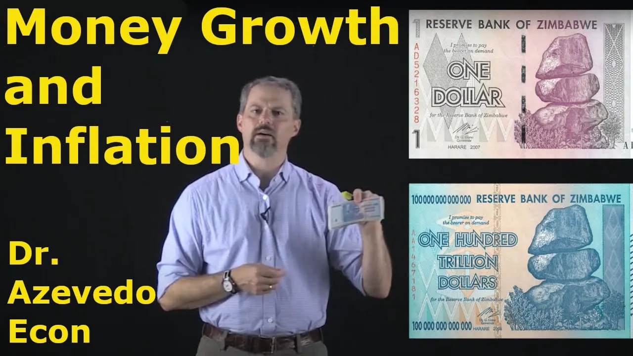


The Quantity Theory of Money states that the equation MV = PY holds, where M is money supply, V is velocity, P is the price level, and Y is real output; when velocity is assumed constant, this reduces to the conclusion that money growth equals inflation plus output growth (mg = π + yG), and in the long run since output returns to full employment (yG = 0), money growth equals inflation (mg = π), demonstrating money neutrality where monetary policy only affects nominal variables like prices and wages without influencing real economic variables such as real GDP or real interest rates.
Quantity Theory of Money: Equation, Velocity & Inflation | Macroeconomics Explained
Added:Understanding the basic definition of money supply (M1 and M2) and how central banks control it.
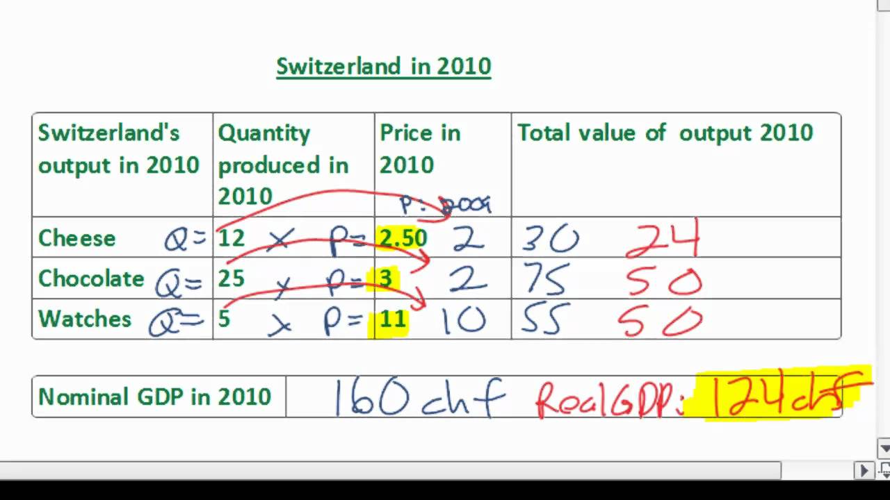
The distinction between Nominal GDP (total market value of goods/services) and Real GDP (output adjusted for inflation).
Basic algebraic skills to manipulate and interpret equations with multiple variables.
Familiarity with the concept of inflation and how the aggregate price level is measured.
The Classical Dichotomy and the breakdown of money neutrality in the short run versus the long run.
The Fisher Effect, which explains the relationship between inflation, nominal interest rates, and real interest rates.
The economic school of Monetarism, specifically Milton Friedman's theories on monetary policy and the stability of velocity.
Historical case studies of hyperinflation (e.g., Weimar Germany, Zimbabwe) and the costs of high inflation (shoe-leather and menu costs).
30.6K views158likes22:52Original Release: 2012-11-08
[Music] morning let's spend a little bit of time talking about the quantity theory of money now essentially this is a classical theory of belonging to the macroeconomics family um it is a very simple relationship of four variables uh and today we're going to understand exactly what what this equation is trying to tell us and the equation that we we're going to look at is is this this see I promise you right it's just four very simple variables um nothing too complicated here uh so let's go through the variables one by one and then I'll tell you a little story about um how they came out with this with this uh equation right here okay now M now m is the um money supply in the economy okay and this is in nominal terms okay um the difference between nominal and real or what they call real balances is basically um this is in value form so how many million dollars or trillion dollars that the economy has uh in in in monetary form um your your real balances or your real money supply is going to be M overp instead so we're not going to talk about that uh keep in mind that this is a uh nominal value and this V over here stands for the velocity now velocity is essentially the number of times Money Changes hand in an economy so let's say in one in one year itself okay uh let's say um there's only two people in this economy you and me and if I got $5 with me and if I use this $5 to buy um I don't know coffee from you uh and and I passed that $5 over to you throughout the entire year that's the only transaction done so that means the velocity of money simply just one okay so in in in short velocity is the number of times Money Changes hands okay okay so so that's for velocity um there's no need to complicate over velocity because uh as you were soon realize we will assume that um the the rate of change of velocity right um the percentage change of velocity is pretty much stable uh so we can actually drop this variable later uh but we'll stick with this first now is the price level okay I think that's pretty straightforward okay the average price level of of your goods um and this is in nominal form obviously okay and now why is output now um a lot of people think that um you know output as you see in your islm model or even ads model they think that Y is actually a nominal um denomination of your of of of goods you know because some people think that it's you know it's GDP Etc but essentially uh when we do macroeconomics or in any other form of theory right um why is actually a real uh denomination okay so it is actually like the total amount of goods and services produced so this is a real value and that is why if you take uh the price level and you multiply that by um the amount of goods services produced by the economy you get the nominal value of um the country's GDP so this two together multiply together you will get the nominal value of your bloody GDP okay so so that's that's um that's something that everybody should take note of when you draw your islm model okay just understand that your horizontal axis represents a real variable and not a nominal variable okay and obviously this side okay is the nominal value of money right so okay not exactly nominal value of money because this is M over here so that's already the nominal value of money so this will be the nominal value of all the transactions done okay okay great so um now I'm going to go into a little story on how this equation was formed um it's not exactly uh the true story but it's kind of like my version of it um okay so we just gonna okay this is a little a little uh scenario that I've drawn out okay we'll go through this one by one okay um there were two friends I haven't given them names yet okay I I'll give them names now okay we'll call this guy John here and we'll call this guy Jack okay all right so the story goes John and Jack you know they are two very um you know enthusiastic entrepreneurs and they had this business idea uh the business idea is simple basically they read this cow they have a cow over here and this cow produces excellent milk okay and uh what they want to do is they want to go somewhere far away H where there's a place where there no cows so that they can sell bottles of milk produced by this cow okay so the place is pretty far away uh the two of then pack their stuff and they bring this carow along and they're going to go there okay um from experience uh this carow at any Tri at any time okay can produce up to a maximum of 10 bottles of milk all right so you got 1 2 3 4 5 6 7 8 9 10 10 bottles of milk okay and they intend to sell each bottle of milk at a nominal fee of $10 okay so essentially how much they expect to make out of this is $100 because you you got 10 bottles multiply by 10 10 bottles multiply by $10 uh they should make a profit of $10 I don't know you know entrepreneurs they are driven by a lot of of of things uh but um something irrelevant but maybe John and Jack they are they're competing over the girl or something like that okay so okay um it's day one and the two of them set off okay so along the journey you know is it's pretty it's a pretty long journey and it's h right so all of a sudden John you know he he feels a little bit thirsty right so you know John John turns around he tells Jack he say hey dude you know I'm I'm feeling kind of thirsty um you know I I happen to have $10 in my pocket right now okay I've got $10 in my pocket you know just my savings um do you mind if I squeeze the cow's tits for a bottle of milk and I'll give you this $10 for it you know just assume I buy it from you so Jack thought that hey that that makes sense I mean you know um at least at least that bottle of be is not g free right okay so John takes his $10 and gives it to Jack okay and you've got one bottle of beer beer of milk that has been bought up by John and John drinks it okay so John is happy and then they start walking and all of a sudden okay Jack starts to get thirsty too so Jack turns to John and he says that hey you know what dude I'm I'm pretty thirsty can I give you this $10 back you know and um let me squeeze a tit of a car so that I can have uh a bottle of uh milk as well so John you know felt the same way and you're okay sure I think that makes sense you know $10 um is is being paid back right so the value of the of the milk bottle you know is paid for so the $10 goes back to John okay and another bottle of milk is gone okay so they keep walking and this happens again and you know what it happens until all 10 bottles of milk has been used up you they they they keep squeezing the tits of the cow you know and 10 bottles of milk is has been um drank drank up already okay and when they reach their destination they realize that there's no more milk left in the cow's TS and they're left with nothing okay so um how does this story relate to the equation that we had okay so here we go we've got mval to p y okay so how much money was there in this simple economy over here that was a piece of $10 note right see there was a piece of $10 note that John was holding on to in his pocket so we've got $10 multipli by the velocity of money okay here's where you will really understand the concept of velocity okay so how many times of this was this $10 exchange between John and Jack okay so when there was one bottle of milk okay this was Exchange once when there's two bottles of milk this was exchange twice three bottles of milk consumed three times four Bott of milk consume four times blah blah blah blah blah so therefore this 10 this piece of $10 was being um exchanged 10 times okay so you've got $10 multiplied by 10 times equals to okay so what is the price level of uh the goods that we are seeing here okay so one bottle of milk was sold for $10 okay and what is output now you understand that output is the total amount of goods and services that has been sold or produced okay and this is a uh real term so we're essentially counting how many products so let's look at the cows whose tits has been uh squeezed throughout the journey um how many bottles of milk did our dear car produce 10 right so essentially 10 bottles of milk is the real output or real GDP right multiplied by 10 units so can you see that this actually makes sense because $100 equals to $100 okay so now this is how the equation makes sense and this is how um some smart guy in the past you know came up with this thing called the quantity theory of of money so now how can we apply this quantity quantity theory of money into uh what we what we study now in the modern times of macroeconomics right okay so I'm going to do some mathematics here just follow me okay so we've got MV equals to py what I'm going to do is I'm going to lawn both sides of the equation so once I lawn both sides of the equation I can actually separate them using the plus sign so I've got lwn M plus lwn v equals to lwn p+ lwn Y okay then after that what I want to do is I'm very interested in the rate of change so I'm going to differentiate with respect to time where time is denoted as a small letter T okay so I'm going to start differentiating now okay once I differentiate this I'm going to get this guy turned around okay and I'm going to have uh D M over DT okay and then same thing for B for V I'm going to turn this guy around and I'm going to differentiate whatever that's inside of the lawn so I'm going to get this okay oh sorry this is a plus here and then same thing for the rest now I'm just going through my motion um we get okay d y over DT okay all right great so now what we want to do is um we want to uh multiply Everybody by DT so that we can get rid of DT okay um multiply by DT and this is what we're going to get we're going to get d m / M plus plus d v/ v equals to this p uh DP over p + y a d y over y okay all right we're almost done now um we're going to make one simple assumption okay we're going to make the assumption that the velocity of money because it is determined by institutional factors um you know such as how much does it cost for you to withdraw money um you know I basically just take this as constant okay so if the change in V okay throughout each time period okay is constant therefore this whole thing equals to zero okay so essentially what we have left is that we have the growth rate of money which I'm going to denote as mg so mg is the growth rate of money this is actually just a simple way of showing it equals to now the change in p over P um for each period that is also known as inflation okay plus the growth rate of the economy YG okay so essentially the quantity theory of money has been reduced to this form over here all right and I'm going to make and no this is not an assumption um this is something that is given um what happens to Output in the long run output in the long run goes back to its original level where full employment occurs so therefore the growth rate of output in the long run essentially this is actually equals to zero so you have your quantity theory of money where um the growth rate of money equals to your inflation rate now so what what what implications you know do we have with this um is simple when your money when the rate of when okay when your money grows your price level is going to grow as well and how much it grows is exactly 141 so if let's say my money my money supply okay is going to increase by 20% a year okay that means inflation is going to increase by 20% a year as well uh inflation is 20% okay uh inflation is not increasing but as in the price level increase by 20% as well okay so now this thing here okay actually explains what we call Money neutrality okay money is neutral neutral okay money is neutral uh that means it has got no effect on any real variables like your real interest your GDP uh okay your real money balances and what have you all the things that is real okay the only things that change are the nominal things like the amount of money you have uh the the wage rate not the W rate but the nominal wage uh so money supply uh nominal wage price level uh nominal interest okay these are the only things that's changed um and the real variables stay the same okay so um how you can apply this you know to to other macroeconomic um models is for example your Adas okay so I'm just going to show you a quick sketch of a Adas okay and this is uh y this is p okay you have your aggregate demand aggregate supply sorry this is Sr okay it's short run aggregate supply and in the long run we know that um everybody just comes back to to why to okay we'll call this um yeah why not okay so this is your long run aggregate supply curve okay so um okay let's go through that one by one okay going to put the price level here okay and um the price level is also equals to the price expectation level of of the of uh laborers okay so now when money supply increases let's say that the government um you know embarks on a monetary expansion efforts um and what's going to happen is that your ad curve is going to shift to the right okay you should brush out your Basics to see why so your ad80 C is going to shift to the right okay this is 81 okay and output is going to go up to y1 and the price level here is now P1 which is more than the uh level of price expectation uh of the laborers right so at this point of time I think you would know that this is a short run and then in the long run what's going to happen is that the uh SES is just going to shift up again okay so um this is what happens okay when uh output increases okay your price level is going to increase because at this point over here okay uh your workers and your machines are actually working over time okay and once they work over time they're going to ask for higher nominal wages okay so uh higher nominal wages okay uh is going to lead to a higher price because when we saw from the price setting model that uh your price level equals to A markup of the wage rate that is being paid to the workers because firms need to earn profit so when this increase this increases therefore this has gone up to this okay so now that's a short run okay now uh we're going to go into the long run okay so we're going to understand how the SRS is going to shift up okay um I'm supposed to explain this in detail in another video but it's okay we'll just do a little bit of that now so the reason why the sras is going to shift up okay is because of another round that your wage rate is going to shift up okay but why does a wage rate shift up again initially we understood that uh you know the real wage uh the real wage the nominal W has shifted up because of this thing but uh recalling your um price sorry your W setting model you have got the real nominal wage equals to your price expectation multip by 1 + a minus uh sorry Z minus Au okay just a recap this is price expectation this is all the unemployment benefits okay uh this is your level of unemployment this is basically a parameter that explains what is the effect of your level of unemployment relating to your weight train okay so now we know that unemployment has dropped okay because now they are working over time unemployment is dropped therefore if this goes down this goes up this goes down this goes up okay so when this goes down this goes up and this releases to this and then for this and this explains a short run now going to the explain a short run here now going to the long run as you can see the price level is more than the expectations of uh price that the laborers have okay so therefore what they want to do is because if they want to keep that real wage okay constant they are going to revise our price expectations so this price expectation here is going to rise up okay this is going to rise up I'm going to use another color because uh this is the long run this is going to rise up uh which caused this to rise up so you know they're going to bargain for higher wages to keep up with prizes so this is going to go up this is going to go up this is going to go up one more time and this is going to go up one bloody more time okay um this is troublesome but just stick with me I think you guys got it already Okay so when this goes up that's where your sres is going to shift up okay so that's why the long run equilibrium is here okay they all stop negotiating until you reach the long run equum point where the real output all the real values are the same your real GDP is the same your real wage is the same your real interest is the same and what have you okay so this is sr1 so essentially the economy has moved like that okay now to apply the quantity theory of money to this is that okay the okay so this is P2 equals to P2 e now you're going to ask me where the P1 where the p P1 go um P1 didn't go anywhere there wasn't any P1 uh I simply put P2 P2 because it just looks nice okay so to explain um how I'm going to use the um quantity theory of money in this is actually a very small step you know you might actually get turn off that you know this video is so long but it's you know you only just uh uh explain one simple part but this is very important because you know um the idea of money neutrality applies to the long run okay so it if you can understand the quality theory of money uh then you can understand you know macroeconomics in the long run so basically this change in price over here or what we call the inflation for that particular year okay is equals to the growth of the money that that the that the government has put in okay so to conclude um monetary policy in the long run has got no effects on the real economy um has only it only has got inflationary um you know implic ations on the economy so that's it okay uh this is the quantity theory of money um I hope you guys enjoyed the video and you enjoyed the um the the story about the car okay so um if you have any questions please uh feel free to please feel free to email me or or drop a comment all right thank you and have a nice day
Up Next
7:14
Austrian Business Cycle Theory | Explaining Economic Booms and Busts
@MarginalRevolutionUniversity
106.3K views•2017-11-28
5:07
Impact of Yuan in Indo-Russian Trade Amid Sanctions
@WION
261.9K views•2022-07-01
10:33
Behavioral Economics Explained: Rationality, Nudges, and Risk
@crashcourse
1.1M views•2016-03-12

113:18
The Age of Easy Money: Fed & Inflation | Full Documentary
@frontline
21.2M views•2023-03-15
Related Study Plans & Knowledge Roadmaps
Structured learning paths in Economics
economics
Sovereign Debt: Defaults, IMF & Restructuring
01Introduction to Sovereign Debt & Government Bonds
02Debt Sustainability & Credit Ratings
03Anatomy and History of Debt Crises
+ 2 more learning modules
12h5 modules
Explore Roadmap
economics
Market Design: Matching Theory & Gale-Shapley
01Introduction to Market Design and Price-Free Markets
02Two-Sided Matching & The Gale-Shapley Algorithm
03School Choice Systems and Mechanism Design
+ 2 more learning modules
10h5 modules
Explore Roadmap
economics
Impossible Trinity: Forex, Capital & Policy
01Introduction to Monetary Policy and Central Banking
02Exchange Rates and International Capital Flows
03The Mundell-Fleming Model
+ 2 more learning modules
8h5 modules
Explore Roadmap
economics
Healthcare Economics: Market Failures & Systems
01Introduction to Healthcare Markets and Market Failure
02Asymmetric Information and Adverse Selection
03Moral Hazard and Insurance Design
+ 2 more learning modules
12h5 modules
Explore Roadmap