



![[BILANGAN KOMPLEKS] : BENTUK POLAR - MENGUBAH BILANGAN KOMPLEKS BENTUK KARTESIUS KE BENTUK POLAR](https://i.ytimg.com/vi/JkYKP6HLakM/maxresdefault.jpg)





![[이얼 대학수학] Stewart 미분적분학 (Calculus, Early Transcendentals) (8판+9판) Part C 제46강 15.2 선적분 (1)](https://i.ytimg.com/vi/tkfOqNxh0R4/maxresdefault.jpg)










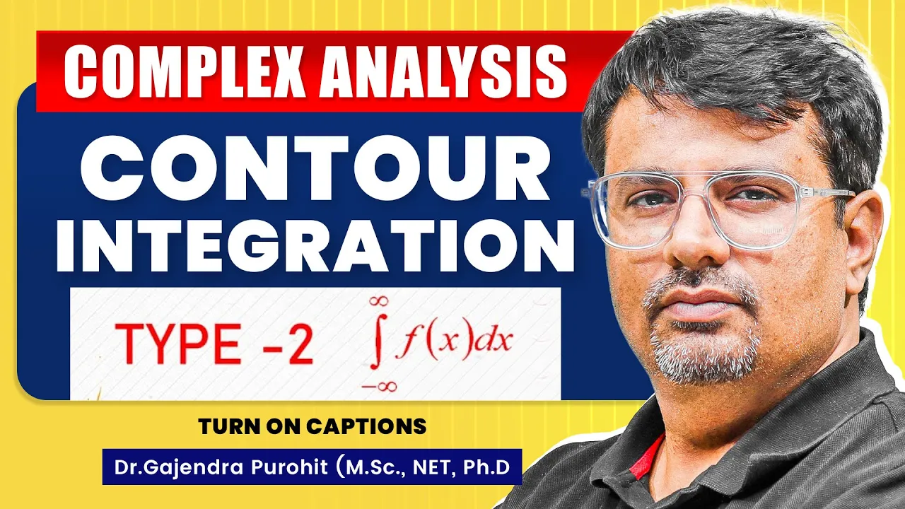
To compute a complex line integral, follow these steps: (1) Draw the curve to understand its geometry and direction, (2) Parameterize the curve using γ(t) = starting point + (ending point - starting point) × t for line segments or γ(t) = re^(it) for circles, specifying the appropriate range for t, (3) Substitute the parameterized curve into the integrand and multiply by γ'(t), then evaluate the resulting single-variable integral using standard calculus techniques.
Complex Analysis: Computing Line Integrals Step-by-Step
Added:Basic complex algebra and geometry, including representation of complex numbers in both Cartesian (x + iy) and polar (r * e^(i*theta)) forms.
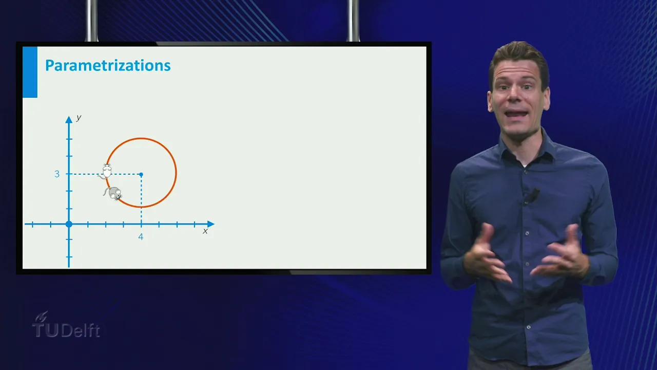
Parametrization of curves in the 2D plane, specifically expressing line segments, circles, and arcs using a single real parameter 't'.
Fundamentals of real-valued multivariable calculus, particularly the concept of line integrals of vector fields or scalar functions.
Definition and properties of complex functions, including the concept of analytic (holomorphic) functions and the Cauchy-Riemann equations.
Cauchy's Integral Theorem, which establishes when the line integral of an analytic function along a closed loop equals zero.
Cauchy's Integral Formula, used to evaluate contour integrals of functions with singularities and to calculate derivatives of analytic functions.
Laurent Series expansion of complex functions and the classification of isolated singularities (poles, removable, and essential).
The Residue Theorem, which provides a powerful tool for evaluating complex contour integrals and finding the values of difficult real improper integrals.
22.3K views282likes7:03Original Release: 2014-08-01
in this video we'll be learning how to compute line integrals so in the previous video we talked a lot about the theory behind it but we didn't actually compute any so let's compute some right now and see how it's done so this is pretty much a step by step process so here's the integral we want to compute we want to compute the line integral of modulus Z squared on the curve gamma and the curve gamma is a line segment from two to three plus I so the first step always always always is to draw your curve even if you know even if you don't think you have to just draw it will help you so here's two here's three plus I and the line segment is like this and as a direction which is we know the direction because it's from two to three plus I and this is our gamma okay so the next step is to parameterize this we need to get an explicit formula for it so remember we talked about how to do this for line segments gamma of T equals the starting point plus something times T and this something is the difference between the ending point and the starting point so three plus I minus 2 is 1 plus I and now we have to also give the range for T which is 0 to 1 so quick check this works right because if we plug in 0 for T we get 2 if we plug in 1 we get 3 plus I so this this will work now the other thing we learned about line integrals is that this is equivalent to the limits of T 0 to 1 and we put in the function so the function in this case is V of Z equals modulus Z squared so we want to put in V of gamma of T into here so that's going to be we put gamma of T in here this is going to be 2 plus 1 plus I times T and I'm going to rearrange this a little bit so I can get real and imaginary parts so I'm going it right this was 2 plus T plus I T ok so that's because I want this real part and this imaginary part it will help because there's a modulus involved so now I'm going to write the modulus of this squared so what is the modulus of this gamma right here so it's going to be radical 2 plus T squared plus T squared and I square that so the square root goes away so it's just going to be the inside part and when I expand this it's going to be 4 plus or T plus T squared plus T squared so it's going to be on in all it's going to be 4 plus 4t plus 2t squared 4 plus 4t plus 2t squared and remember we need to multiply this by gamma prime so we need to take gamma prime of T equals and this is why I split it into two components so it's going to be 1 plus I 1 plus I so 1 plus I DT and the reason I'm able to write it like this so go back to the previous video on the theory over line integrals if you want to real quick refresher on why I'm allowed to do this but we talked about how you can transform a line integral into something that just involves T something it's much easier for us to compute so the form is again limits of T you take the function you plug in the gamma you write gamma Prime and then DT so now this know a piece of cake we can evaluate it so this 1 plus I is just a constant we can take it to the outside and we're going to evaluate this inside integral it's going to be 40 plus 2t squared plus 2/3 T cubed limits the 0 to 1 so we plug in 1 into all this we get 4 plus 2 plus 2/3 is 6 plus 2/3 is what 20 thirds and don't forget the 1 plus I we had taken outside so this is 20 thirds 1 plus I that is the value of the line integral so just to recap the process is always draw a graph always always draw a graph parameterize the curve in explicit formula and then just plug everything in the equation after you take the derivative and stuff like that and then work it out using your normal calculus techniques we'll do one more here on the back so to get a different curve this is going to be we won the line integral of Z squared on the curve gamma and the curve gamma will be a semicircle from 1 to negative 1 through I so remember always first draw the graph here's one here's negative one and the semicircle through I so here's I so the semicircle is going to look like this and what's the direction of travel well it says from one to negative one so the direction of travel is this way ok so next step is to parameterize this what's the gamma formula remember we said for circle it's going to be radius so right the one even though I really have to one times e to the I T and that's the formula and T's range we have to be careful here because in the previous video we talked about the range being from zero to 2pi but that's what we want the full circle since we stopped at the halfway mark this starts at zero and it goes to the angle PI so T's range is 0 to PI ok you got to be careful with your ranges be careful with your parameter ization this is actually the hardest part once you figure that out you know it's good then you just do calculus techniques it should be good from there so now let's write the integral in the form we have integral so limits now of T and then what's the what's the function the function is Z squared so I want to take the gamma and square it so it's going to be e to the 2i t e to the 2i t and now order to gamma Prime so gamma prime of T is going to be I'm going to take the I down so then be I e to the I T okay so you just treat I like a constant when you take integrals derivatives stuff like that so now we plug that in here I'm going to take the I outside because it's a constant and we're going to have e to the I T DT so now these two can multiply together so I zero PI e to the three I T DT now this we can work out so it's going to be I times 1 over 3 I eetu the 3i t limit 0 to PI ok so let's work this out this I and this I can cancel so just going to be really one-third and it's going to be e to the 3 I PI minus e to the 0 e to the 0 we know is 1 so it's going to be 1/3 eetu the 3 PI I minus 1 so what is e to the 3 PI from the exponential video we know we can write this thing as cosine 3 PI plus I sine 3 PI sine 3 pi is 0 cosine 3 pi is negative 1 so this is going to be negative 1 minus 1 times 1/3 it's going negative 2/3 so interesting this has no imaginary component but answer on the back did have an imaginary component so you see this is really not that hard to work out you just got to be very careful in two steps the first thing is drawing the graph make sure you understand what the gamma is the second thing is writing the parameter is a ssin if you have to look at it plug in different T values and make sure it works but once you have these two things solid you're good then you just put everything in the form that we had in the previous video and then you just work through and you should get a nice answer in there okay
Up Next
40:45
Complex Integration & Cauchy's Theorem | Residue Theorem Explained
@mathemaniac
436.6K views•2022-01-22

4:43
Elliptic Curve Cryptography Explained: ECC, ECDSA, ECDH
@PracticalNetworking
28.5K views•2024-10-21

18:15
Metropolis-Hastings Algorithm: MCMC Sampling Explained Simply
@ritvikmath
138.8K views•2021-01-25

6:00
The Mathematical Impossibility of Accurate World Maps
@Vox
23.3M views•2016-12-02
Related Study Plans & Knowledge Roadmaps
Structured learning paths in Mathematics
mathematics
Tensor Calculus: Vectors to Riemann Curvature
01Mathematical Foundations: Linear Algebra & Calculus
02Covectors, Dual Spaces, and Tensor Basics
03The Metric Tensor and Index Gymnastics
+ 2 more learning modules
40h5 modules
Explore Roadmap
mathematics
Gödel's Incompleteness: Logic, Proofs & Limits
01Introduction to Formal Systems & Hilbert's Dream
02Set Theory, Cardinality, and Cantor's Diagonal Argument
03Arithmetization and Gödel Numbering
+ 2 more learning modules
14h5 modules
Explore Roadmap
mathematics
Galois Theory: Fields, Groups & Solvability
01Foundations of Abstract Algebra: Groups & Fields
02Polynomials & Field Extensions
03Splitting Fields & Symmetries
+ 2 more learning modules
24h5 modules
Explore Roadmap
mathematics
Non-Euclidean Geometry: Models & Geodesics
01Euclid's Fifth Postulate and the Birth of New Geometries
02Hyperbolic Space and the Poincaré Disk Model
03Geodesics: Defining Straight Lines in Curved Spaces
+ 2 more learning modules
15h5 modules
Explore Roadmap