Metropolis-Hastings Algorithm: MCMC Sampling Explained Simply

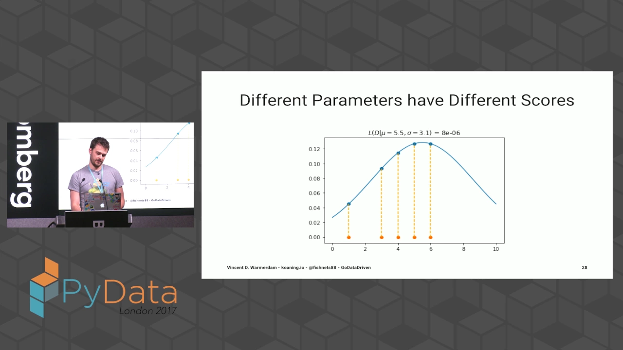
[00:00:00][Music] hey everyone how's it going so today we're going to be talking about the most popular mcmc algorithm called metropolis hastings so again our goal in all of this is always to sample from some kind of distribution p of x and as we've been assuming in the sampling videos we don't know the exact form of p of x as is common we only know the numerator f x which is this blue line up here so in explicit mathematical terms p of x is equal to f of x divided by some normalizing constant that is difficult to compute so the question is again can we use only f of x in order to get samples from p of x and the way mcmc tackles this problem is to design a very special type of markov chain such that the initial samples that we're getting which we're going to call the burn-in period may not exactly follow the target distribution p of x but eventually we're going to get to some kind of sample x b some kind of state in the markov chain xb such that everything from there on is going to be treated as a sample from p of x so this initial part is called the burn-in we typically throw those away because they're not following the distribution but are necessary in order to get to a point where from there onward we are sampling from the distribution and so that was all said in our initial mcmc video linked in the description below but uh the big question we had there is how exactly do we design these transitions these transition probabilities from one state to the state that comes after it and metropolis hastings goes about it in the following way so just like with accept reject sampling we are going to propose some kind of candidate so we're going to again begin by saying that hey this is a possible candidate that you might want to consider except here's the first difference in accept reject sampling that sample was independent that candidate was independent so we typically had for example a normal distribution with some kind of fixed mean some kind of fixed standard deviation and we kept getting candidates from that now we're not doing that here because we know explicitly that the next sample is going to depend on the sample before it so instead of having the mean be fixed we are going to have the mean of this normal distribution be exactly the previous sample that we considered and now just to backtrack for a second what we're doing generally is that we're trying to get some kind of easier distribution to sample from g so typically for us that's been the normal distribution but it doesn't have to be it can be any distribution such that it's easy to sample from and its domain is the same as your target distribution and so we're saying that we want to sample the next sample x t plus one from that distribution but it's going to be dependent on the sample that came before it x t so this form right here is exactly respecting the form of the markov chain and so for us we're going to say that this is going to be the normal distribution centered at the previous sample x sub t and with some fixed variance sigma squared so in more easy terms we're saying that go look at your previous sample which is x sub t center a normal distribution there at x sub t and then sample the next candidate x sub t plus 1 exactly from that normal distribution so that's a picture you're looking at here and so like i said before we don't have to use the normal distribution we can use any distribution we want as long as it follows the conditions we talked about so you can even use this asymmetric distribution that looks like this so this would be your x sub t and you sample your next candidate from this distribution now the choice of whether this distribution is symmetric like the normal distribution or asymmetric like this distribution here does matter in the naming so you might have heard metropolis hastings algorithm versus just metropolis algorithm and here's where that difference comes in the metropolis algorithm so dropping the hastings is if your candidate distribution is symmetric like the normal distribution metropolis hastings is the more general case that encompasses the metropolis algorithm but also all situations where your candidate distribution can be asymmetric like this one here and that matters because now let's say you sample your next point x sub t plus one so let's say that's here and let's say you accept that sample which that's what we'll talk about next but let's say that's your next sample then if it's symmetric that's saying that you have just as much of a probability given that you end up at x t plus one to go back to x t because notice that this probability here of going from x sub t plus one and proposing x sub t is the same as this here so they're symmetric with the asymmetric case that is not generally true so we see that if we're at x t then the probability of proposing x sub t plus one is around here however if we're at x sub t plus one the probability of proposing x t is clearly different down here so different in naming but besides that the algorithm is going to work in the same way the metropolis case just simplifies our math a little bit too as we'll see in a second but either way step one as we said is just take some easier distribution to sample from the normal distribution for example and propose a candidate for the next state of the markov chain now i want to be very clear here that that is not the definite next sample this is just our candidate this is we're going to ask if we should accept or reject this next state and that brings us to step two which is we're going to accept this next state x sub t plus 1 with some probability given by a a for except going from x t to x t plus one okay so it's a two-step process pretty simple at a high level we first propose some kind of next sample based on the previous sample and then we choose to accept it with some probability here and so the lingering question of course is how do we define this acceptance probability a we're going to go back to our old friend the detailed balance condition so i talked about that in the initial mcmc video and what i said was that if we can show that the probability of going from any state x sub t to any next state x sub t plus one follows a detailed balance condition then we're golden we know that p of x will be a stationary distribution of the markov chain and therefore eventually the markov chain will be sampling from p of x and so here's the detail balance condition it basically says that for any states a and b so any a and b you can see on this x axis we need for this condition to be true p of a times the transition probability of going from a to b must be equal to p of b times the transition probability of going from b to a that's the detail balance now let's plug in some things because we can simplify a lot of these things based on what we talked about here p of a based on this equation here is simply f of a divided by the normalizing constant we do this because we don't actually know how to compute p of a but we know how to compute f of a so that's f of a over nc and for the same reason that's f of b over nc on the right hand side now let's stop and think what is the probability given that i'm currently at state a of going to state b next well it's a two-step process the first one is i have to be proposed state b by g so that's what you're seeing here i have to be proposed state b given that i'm currently at state a and then i have to accept that proposal which happens with a going from a to b so what is the probability of accepting a proposal going from a to b so again this first part is what's the probability it's proposed at all that is this part here and the next part is given that that's the proposal what's the probability that i accept it and do actually go to that next state and that is this guy here and we see the same terms here just with a and b's roles reversed so we're going to follow this arrow up here it looks like this is getting a little bit convoluted but we're going to see how it simplifies real nice we're going to collect all the acceptance probabilities on the left hand side as a ratio so if you restructure this equation you'll pretty easily see you can get to that equation there which is acceptance probability of going from a to b divided by the acceptance probability of going from b to a is equal to f of b over f of a times g of a given b divided by g of b given a and just to simplify these terms in our mind we can call this r sub f which is ratio of f and we can call this r sub g which is ratio of g so we see this has a very nice symmetry there are clearly three different terms that are going on here and now this is the definition that metropolis hastings gives for these acceptance probabilities up here i'm just going to give them to you first and then we're going to check that they work and then at the end we're actually going to show the intuition behind why this is why you would want to do this metropolis hastings says that if rf times rg which is this right hand side of the equation is smaller than 1 then acceptance of going from a to b is rf times rg and first note that this is good because we need to interpret this acceptance as a probability so it needs to be bounded between zero and one and we know that this guy is bounded between zero and 1 because that was our condition for this case so okay so far and we say that acceptance of going from b to a is going to be exactly 1. let's make sure that this obeys this detailed balance condition up here so if rf times rg is less than one then our numerator is rf times rg and our denominator is one that means that the left hand side is simply rf times rg and the right hand side is by definition rf times rg so good to go satisfies detailed balance now the other case of course is what if rf times rg is bigger than or equal to one then the acceptance of going from a to b is going to be exactly 1 and the acceptance of going from b to a is going to be 1 divided by rf times rg which is a valid probability because this guy was bigger than 1 so its reciprocal has to be less than 1 and therefore its reciprocal can be interpreted as a probability let's do the same sanity check so if i plug in 1 here and i plug in 1 over rf times rg then the reciprocal flips and the left hand side is again equal to rf times rg which is by definition the right hand side so we've done a lot of talking here but we can actually collect all these thoughts into a single equation and if you noticed a small blip on the board i had to change something so please excuse that so we can collect all these thoughts we just said into this equation that says that the acceptance probability of going from a to b so you're at state a right now what's the probability that if you propose state b next you actually accept that move is going to be equal to the minimum of 1 and rf times rg quick sanity check if rf times rg is less than 1 then the minimum of 1 and that quantity is going to be that quantity it's less than 1.

[00:10:58]and that's exactly following this definition up here however if rf times rg is bigger than one then the minimum of one and that quantity is going to be one and that again obeys the condition here so we see that all this logic we went through can be coalesced into this single equation and that single equation is saying that if you're currently at state a and you're trying to figure out if i should accept the move to state b then you can do it by setting your acceptance probability according to this rule and now let's pause for a second and review the algorithm itself because we've done a lot of talking we've done a lot of derivations it can be easy to lose sight of what we're actually doing i'm going to go through the algorithm again pretty quickly and then most importantly to close this video i'll be giving you an intuition because i realize this is all just math so far the algorithm says that if you're currently at some state x sub t step one is to sample from this easier distribution g for example normal distribution sample your next candidate from that distribution so now you're holding on to this candidate and you're trying to answer the question of should i accept it or not step two says that we are going to accept that candidate based on this acceptance probability minimum of 1 and rf times rg which is again these terms up here so you take the next state that you've been proposed plug that in as b you take the initial state you're at you plug that in as a you compute these guys and notice you can compute all these things because you have f and you have g so there's no issues about needing p anywhere here so you compute that you get the minimum of that quantity and one and you set that as your acceptance probability and we showed that this satisfies the detailed balance condition and therefore it does lead to p being a steady state or a stationary distribution for your markov chain and so eventually you will be sampling from this distribution p after some burn-in period and the last part of the story is that if you don't accept the sample so this is your acceptance probability of going from a to b so let's say that you do accept it that means that the next state in your markov chain is indeed b because you accepted it however if you do not choose to accept b then the next state in your markov chain is simply just the previous state carried forward so you basically stay where you're at and take the same sample you just took again and then you try again for the next round okay so that's the mechanics of how it works but let's end this video by talking about why the heck does this actually work because if you're like me this is not a satisfying answer to the problem so here's the intuition for the intuition let's uh default to the metropolis case it'll just be easier for us to talk about everything and the metropolis case says that g of a given b is the same thing as g of b given a because that is what's implied by the symmetric nature of our candidate distribution and that means that these guys just cancel out and that's equal to one so actually the acceptance probability of going from a to b is simply minimum of one and just rf because rg would be one in that case and rf is equal to f b divided by f a and we know that rf so f of b divided by f of a is actually just p of b divided by p of a because they are proportional only up to this normalizing constant so we have the acceptance probability of moving from a to b so accepting a move from a to b is given by the minimum of 1 and p of b divided by p of a now to truly understand why the metropolis algorithm works and what it's trying to do let's split into two cases the first one is that the probability of b is bigger than the probability of a and before going on let me draw that for you let's say that we're currently here so this place is a where we're at right now and let's say the next place we've been proposed to go to by our candidate distribution is this b here so we're trying to figure out if we should accept that move or not and now if p of b is bigger than p of a which is the case here p of b is clearly a more probable state than p of a according to our target distribution then this minimum is going to give us back one and so it's saying that there's a hundred percent chance that you're going to be at b for your next state and that makes sense because what we're trying to do what metropolis algorithm is trying to do is saying that if the next place you're trying to go is more probable than the current place you're at you are 100 going to accept that move so in a nutshell it's kind of allowing us to inch towards higher and higher and higher densities of our target distribution which would be around this area here where it's the most probable and this is the beauty of the metropolis algorithm or metropolis hasting algorithm is that it is allowing us to move incrementally closer to areas of high probability something that the accept reject method simply just did not do because each sample was independent of the last so metropolis algorithm says that look where you're at right now look where you're being proposed to go if the place where you're being proposed to go is a high density area of your target distribution you better go there we need more samples from there and looking at the last case if probability of b is less than probability of a so let's say b was instead over here which is a lower probable region than the initial state a so we're asking if this is a move that i want to make then the acceptance of going from a to b is going to be probability of b divided by probability of a again just inferring from this minimum function right here and so probability of b divided by probability of a is going to be less than one by definition by this condition and therefore we still might go to that lower density area but it's just not a hundred percent probability and more interestingly the bigger the gap between this lower density area and the current place we're at the less likely we are to go there for example suppose that this was one half that means that the place we're trying to go is half as probable as the place we are right now then there's a 50 50 shot we would go however if the place we're trying to go is like a hundred times less likely than the current place we're at this is going to be 0.01 and therefore there's a very low chance of going there so intuitively what the metropolis algorithm is aiming to achieve is that no matter where we're at no matter where we're being proposed to go we are going to accept that move if that is a more likely place to be because we want more samples from these high density areas and we might accept the move if it is a low density area and we need this to be mite because we still need to sample the tails it's still important of course for the distribution but it's just not as important as sampling the main body of the distribution where most of the density is at so i know this was kind of a long video um i wanted to do it justice because this is such a cool method i wanted to show all of the power of this method intuitively why it works mathematically prove that it works to you um so there's no question in your mind when i first learned this it was kind of magic i wasn't sure exactly what's going on so i don't want it to seem like magic for you so this is the metropolis hastings algorithm how it works the math of it into edition so if you like this video please like and subscribe for more videos just like this i've gotten lots of comments to walk away from the board so you can look at everything so that's what i'll do now see you next time