




















![[PLDI'23] Probabilistic Programming with Stochastic Probabilities](https://i.ytimg.com/vi_webp/dYHKSHjbxFY/maxresdefault.webp)

Gibbs sampling is a Markov chain Monte Carlo method for sampling from multi-dimensional probability distributions by iteratively sampling each variable from its conditional distribution given the current values of all other variables, accepting all proposals without rejection; unlike the Metropolis algorithm, it requires knowing the conditional distributions and being able to independently sample from them, making it particularly useful for Bayesian inference but potentially less efficient when parameters are highly correlated.
Gibbs Sampling Explained: A Practical Introduction with Examples
Added:Joint, marginal, and conditional probability distributions, especially in a bivariate context.
The fundamentals of Bayesian inference, including priors, likelihoods, and posterior distributions.
Basic Markov Chain theory, including states, transition probabilities, and the concept of a stationary distribution.
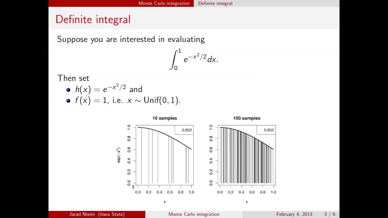
The general concept of Monte Carlo integration and why sampling is used to approximate complex integrals.
The Metropolis-Hastings algorithm, which generalizes Gibbs sampling for cases where conditional distributions are difficult to sample directly.
MCMC convergence diagnostics, such as monitoring trace plots, calculating autocorrelation, and using the Gelman-Rubin statistic.
Applying Gibbs sampling to complex models, such as Latent Dirichlet Allocation (LDA) and Hierarchical Bayesian models.
Using modern probabilistic programming languages (such as PyMC, Stan, or JAGS) to automate and scale MCMC sampling in practice.
86.1K views1.3Klikes18:58Original Release: 2018-05-15
in this video I want to provide a short introduction to Gibbs sampler so what is Gibbs sampler so it's a way of sampling from probability distributions of two plus dimensions and like the metropolis algorithm it is a method of Markov chain Monte Carlo so that means it's a type of dependent sampling algorithm however unlike the metropolis algorithm we accept all proposals indeed it is possible to show that the Gibbs sampling algorithm is a special case of the metropolis algorithm and vice versa and the Gibbs sampling algorithm is again like the metropolis algorithm often used in Bayesian inference and it is actually the kind of method that underlies the bugs and jagz languages in order to explain what is meant by gibbs sampling i'm going to use an example and then hopefully through the example you should see kind of how this process works and then afterwards i will formally define the algorithm so the example we're going to use is the case of horse racing so we imagine that there are two horses a and B and they race on the same day but in separate events and those horses can either win the event in which case their particular random variable is equal to one or they don't win the event in which case their random variable is equal to 0 and we suppose that there is this joint probability distribution of a and B further suppose that what we want to do is to sample from this joint distribution so what do I mean by sample from this joint distribution well what we will be doing is we would be generating sequences of paired outcomes so here we might first of all sample a value of 0 0 the first 0 indicating that horse a did not win its race and the second 0 also indicating the horse B did not win its own race and then we might sample 0 1 then say 0 1 again etc so we generating sequences are paired event it where each of the pairs that we sample has a probability that's given by this table here so the probability of a and B both losing is given by the top-left corner and that's a 0.1 probability so there is a simple way to generate independent samples from this joint distribution which is to take the unit interval and basically chop it up so that this first quadrant here is of area 0.1 then we have the next area which is say 0.4 so this would be the next area and the first area 0.1 here would correspond to a 0 0 event so both forces losing then we have the 0.4 of M which is corresponding to when a wins but B losses and then we chop up the last two bits according to naught point three and no point two two correspond to the other two cases in our table then what we do is we generate a uniform number between 0 and 1 and we basically figure out which of these compartments it falls in and whichever compartment it falls in that corresponds to a particular head set of outcomes however what I want to illustrate in this video is how we can use a different method which is give sampling to enable us to sample from this joint distribution and whilst it seems more complicated than their simple method that I've outlined just now for this simple case in more complex examples you can't use simple rules like the one I've just highlighted especially for continuous parameters so what Gibbs sampling relies on us knowing are the conditional distributions and being able to independently sample from those conditional distributions so firstly what we're going to do is we're going to figure out what the conditional distributions of a conditioned on particular values of B look like so we're going to have two different conditional distributions here one where we're conditioned on the fact that B equals 0 and the other where B is equal to one so if B is equal to zero then essentially if we look back at our joint table that is corresponding to these two outcomes here so our new probability space essentially collapses just to this row so because it collapses down to this row what we need to do is we need to normalize each of these values by the sum of the entries of the rope so the sum of row entries here are just not point five so to work out the probability that a equals zero given that B equals zero then we just take this 0 point 1 value and we divide it through by the row sum so we just get 1/5 and then for the other term in this conditional distribution so when we're conditioning on B being with a 0 we take the zero point four value and then we divide it through by 0.5 so we get 4/5 so we noticed that this row here is a valid probability distribution now what we're going to do is we're going to create a different valid probability distribution where we condition on B being equal to one so when B is equal to one we are just restricting ourselves to this bottom row case here in which case what we need to do is again we need to renormalize so we divide each of the corresponding probability values through by the row sum so firstly we get a value of 3/5 so that's just no point three divided by 0.5 and then we get two bits so again we get a valid probability distribution in this bottom row now what I want to do is I want to do the same but I want to generate the probability distribution or be conditioned on a so now we're going to be looking at the columns whereas before we were looking at the roads so now suppose that we're conditioning on the fact that a is being equal to zero then if we look back at our joint distribution that is corresponding to these two set of values here so what we need to do is we need to divide through each of these values by the sum of that column so here we just sum them together and we get north point four and we might as well do it for the other column because we're going to need it in a minute if we sum these two values together we get 0.6 so firstly for the probability of B condition on a being equal to zero to get those values we divide not point one by not point four and then we'll divide not point three but not point four so first thing we get one quarter and then we get three quarters so we notice that in this column we have a valid probability distribution then we do the same thing but in the second column so now we're conditioning on a being equal to one and so we're going to divide each of these values by the respective column son so firstly we get no point four over nor point six which is just 2/3 and then we getting off point to open or point six so we get 1/3 so we notice that we have four possible conditional distributions we have the probability distribution of a conditioned on B being equal to zero we have the probability distribution of AE conditioned on B being equal to 1 we have the probability distribution of B conditioned on a being equal to zero and we have the probability distribution of B conditioned on a being equal to one and basically because there are only two outcomes for each of these conditional probability distributions it's in effect the same probability distribution as flipping a coin albe it's one which has some bias so for example if we were considering the probability distribution of a conditioned on B being equal to zero that would be like throwing a coin where the probability of heads was given by four fins and let us suppose that as is the case with I think most statistical software we are able to computationally simulate throws of such a bias coin now what I'm going to do is I'm going to show you the results of simulations of the Gibbs sampling algorithm for this example so what does the give sampang algorithm look like here well first of all we start off by sampling a value of a and B from some arbitrary probability distribution which has support over the allowed values of a and B in other words it only generates a being equal to 0 or 1 and similarly for B then what we do is we iterate for iteration T in 1/2 large T here we do the following firstly we sample a value a from the conditional probability distribution of a where we condition on B the previous value of B that we sample then what we do is we use this value of a that we've just independently sampled to define a conditional probability distribution of B where we condition on a t and we sample from be there and we independently sample B from this distribution so notice what we're doing here we're using the previous value of B in the previous iteration to define a conditional probability distribution for a that we independently sample from then we use that value of a to define a conditional probability distribution for B and we sample be from that independently so now what I want to do is I want to illustrate this process visually so I have these four possible outcomes represented by these four dots on the screen here and here I just so happens to have sampled a value of zero zero as my starting point then what we're gonna do is begin to update a by using the conditional distribution of a when B is equal to zero because first of all starting off would be being equal to zero and the corresponding probability distribution of each of the possible values of a I've shown above each of the values of a so this value here if you look back in the table is 1/5 and this value here is 4/5 so we're going to independently sample a value of a from that and if we do so it happens that we pick a being equal to one so we move that then what we do is we update B only sampling from the probability distribution of B conditioned on a being equal to one so now we're choosing between each of these two dots here and the corresponding conditional probability distribution is shown to the right of each of these dots and if you look up these values in the table this one here is 1/3 and this one here corresponds to 2/3 so if we carry out that independent sampling turns out that we move here in this case to a and B being equal to 1 then what we do is we do the same thing for a so now we're choosing between each of these two dots here and notice the the conditional distribution that we're drawing from this time is different to what we drew from last time when we were drawing for a because now B is equal to 1 so the conditioning on B being equal to 1 whereas previously we were conditioning on B being equal to 0 and we move again and we essentially then iterate this process so now I'm going to do the same for B what do we do and move again for B and we continue this process over and over again and what we kind of see is if we iterate this process continually and we look at the number of values which we've sample from each of these locations then eventually we will see that we approximate the underlying joint probability distribution now I want to back up just what I said by showing that if we continue to iterate these 2 steps that eventually our sampling distribution approximates well the truth Joint Distribution so now what I'm showing by the area of the black dots is the true joint distribution and the pink areas that currently is just on the a and B because a 0 case because I'm starting here are the sampling distribution values and so what we can see is as we run this algorithm the the sampling distribution soon starts to well approximate the true underlying probability distribution which is given by the black dots and so the after we run a few thousand iterations here we get a very good approximation and in fact after 10000 iterations it's very hard to tell the difference between the true distribution which is the black dots and the pink ones because essentially they're just exactly the same size so you've seen here that 10,000 iterations from this algorithm results in a sampling distribution that well approximates the joint now that I've Illustrated the Gibbs sampling works for this two dimensional discrete distribution I want to formally define it so I'm going to define it using a three dimensional probability distribution which may be discrete it may be continuous of three parameters theta 1 theta 2 and theta 3 so here we're supposing that what we want to do is to generate samples from this three dimensional probability distribution in Gibbs sampling like in metropolis we first of all starts off by sampling some values of theta 1 theta 2 and theta 3 randomly from some arbitrary probability distribution which is simple to draw samples from but still has support over the allowed values of theta 1 theta 2 and theta 3 then what we do for iteration little T in one two big t is firstly there is sometimes a randomization step here where you randomize the order in which you're going to do the updating but that's not essential so I'm going to leave that out for the time being so we're going to imagine that we're going to update theta one then theta 2 then T 2 3 in each of the iterations here because I've chosen a non randomized parameter update order so firstly what we're going to do is we're going to sample a value of theta 1 from the conditional distribution of theta 1 where we condition on theta 2 in the previous iteration and Pisa 3 in the previous iteration so independently sample of value of theta 1 from this conditional then what we do is we do the same for theta 2 but we use the just recently produced value of theta 1 to define a conditional probability distribution so now we sample a value of theta 2 conditioned on theta 1 T and theta 3 t minus 1 then what we do is we use the recently produced values of theta 1 and theta 2 to define a conditional probability distribution which we sample from for theta 3 so we condition here on T 2 1 T and theta 2 T so like random walk metropolis under quite general conditions this algorithm is guaranteed to automatically converge to the target distribution here the joint probability distribution of theta 1 theta 2 and theta 3 however you'll notice that the requirements of this algorithm starting more stringent than that for random walk topless however unlike random walk metropolis you'll notice that there is no accept rejected we're just accepting all of our proposals they're all just sampled from the respective conditional probability distribution and so because we don't reject any proposals Gibb sampling in general is more efficient of exploring parameter space than random walk metropolis however the conditions to be able to use this algorithm or more stringent than for random walk metropolis we need to know what each of these conditional probability distributions is and we need to be able to independently sample from and in general finding this conditional probability distributions can be difficult or impossible for many applied examples also another problem with Gibbs sampling which is also a problem for random walk Petropolis is that it can be very slow for correlated parameters and the reason for that is that if we've got two very correlated dimensions here in other words the probability distribution is very correlated so imagine we can represent that by a contour plot which looks something like that which I'm drawing now then the conditional probability distributions actually aren't that wide so for example if we condition on a value of theta2 which is somewhere like that then typically the values of theta one that we draw from are somewhere in here because of the correlation in the parameters that means that Gibbs sampling tends to do quite a slow sneaking path across posterior space that will look something like this pink line that I'm drawing here and because of this sneaking way in which it moves up a diagonal landscape it actually takes Gibbs sampling a long time to explore posterior space when we have a high degree of correlation between parameters here what we don't dearly like to do is walk in the diagonal direction random walk metropolis does allow you to walk in that diagonal direction but unfortunately it proposes values that are frequently off of that diagonal so we only accept a very small minority of cases where as we shall see later on that Hamiltonian Monte Carlo actually allows us to get the best of both worlds we can walk in the diagonal direction and we accept a high proportion of steps in situations where we have highly correlated parameters it can actually make a lot of sense to use Gibbs sampling update in blocks of parameters where the blocks correspond to those parameters that are highly correlated with one another so suppose the theta 1 and theta 2 are correlated with one another then what we want to do is we'd want to sample from the conditional distribution of theta 1 and theta 2 conditioned on theta 3 and it will turn out that this sampling method in general is more efficient than just something from the uni-dimensional conditional distributions but unfortunately much like we can't always derive conditional probability distribution especially univariate it's generally harder to find ones which are multivariate so this is even harder in general than deriving the univariate rules that we've needed so far so in summary give something is a way of sampling from a two plus dimensional probability distribution it's a variant of Markov chain Monte Carlo and it requires us to know the conditional probability distributions it can be much much more efficient than random or metropolis exploring posterior space because we don't reject any steps however it does require us to know the conditional probability distributions and be able to independently sample from them both of which may be difficult in practice
Up Next
52:47
Bayesian Modeling in R with Stan | A Gentle Introduction
@slcrug
42.5K views•2018-11-15

4:43
Elliptic Curve Cryptography Explained: ECC, ECDSA, ECDH
@PracticalNetworking
28.5K views•2024-10-21

10:44
Fourier Series Introduction: The Big Idea Explained
@DrTrefor
387K views•2021-05-03

6:00
The Mathematical Impossibility of Accurate World Maps
@Vox
23.3M views•2016-12-02
Related Study Plans & Knowledge Roadmaps
Structured learning paths in Mathematics
mathematics
Tensor Calculus: Vectors to Riemann Curvature
01Mathematical Foundations: Linear Algebra & Calculus
02Covectors, Dual Spaces, and Tensor Basics
03The Metric Tensor and Index Gymnastics
+ 2 more learning modules
40h5 modules
Explore Roadmap
mathematics
Gödel's Incompleteness: Logic, Proofs & Limits
01Introduction to Formal Systems & Hilbert's Dream
02Set Theory, Cardinality, and Cantor's Diagonal Argument
03Arithmetization and Gödel Numbering
+ 2 more learning modules
14h5 modules
Explore Roadmap
mathematics
Galois Theory: Fields, Groups & Solvability
01Foundations of Abstract Algebra: Groups & Fields
02Polynomials & Field Extensions
03Splitting Fields & Symmetries
+ 2 more learning modules
24h5 modules
Explore Roadmap
mathematics
Non-Euclidean Geometry: Models & Geodesics
01Euclid's Fifth Postulate and the Birth of New Geometries
02Hyperbolic Space and the Poincaré Disk Model
03Geodesics: Defining Straight Lines in Curved Spaces
+ 2 more learning modules
15h5 modules
Explore Roadmap