


















Bayesian inference reverses conditional probability using Bayes' theorem to update beliefs about parameters from data, treating parameters as random variables with probability distributions rather than fixed unknowns; Stan is a probabilistic programming language that implements Markov Chain Monte Carlo methods to sample from complex posterior distributions, enabling practical Bayesian analysis through hierarchical modeling and flexible prior specification.
Bayesian Modeling in R with Stan | A Gentle Introduction
Added:Basic proficiency in R programming, including data manipulation, installing packages, and writing simple scripts.
Fundamental understanding of probability theory, specifically probability distributions, joint/conditional probabilities, and Bayes' Theorem.
Familiarity with standard statistical modeling, such as classical linear regression and the concept of parameters.
A conceptual understanding of the difference between frequentist statistics (fixed parameters) and Bayesian statistics (parameters as random variables).
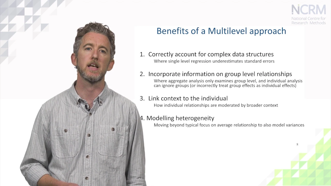
Mastering Bayesian Hierarchical (Multilevel) Modeling to handle nested or grouped data structures.
Advanced MCMC diagnostics and troubleshooting, including identifying and fixing divergent transitions, checking R-hat, and assessing Effective Sample Size (ESS).
Bayesian model evaluation and comparison using Posterior Predictive Checks (PPCs) and information criteria like WAIC and Leave-One-Out Cross-Validation (LOO-CV).
Exploring high-level R interfaces for Stan, such as 'brms' and 'rstanarm', to build complex models with simpler syntax.
42.5K views1.1Klikes52:47Original Release: 2018-11-15
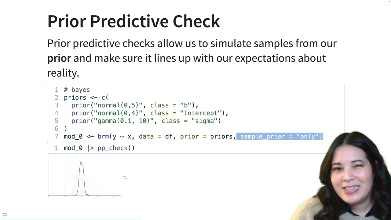
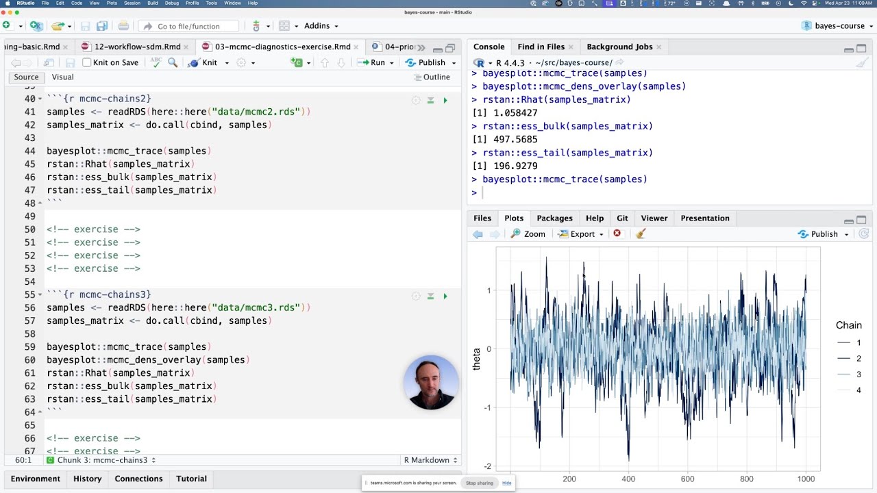
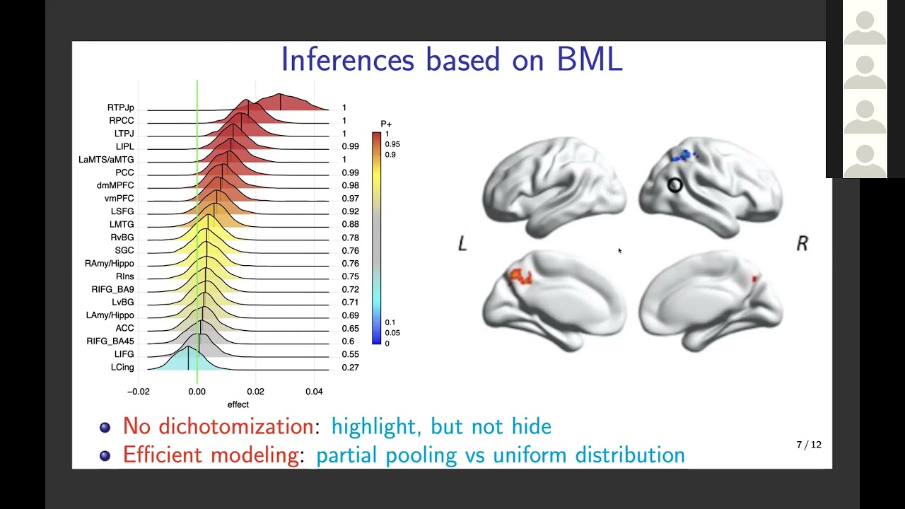
all two would be like you've dabbled you kind of understand the basic philosophy but you don't really do much Bayesian modeling on a regular basis three would be yeah I use this all the time so how many ones do we have in here like no experience at all never hardly even heard of it okay how many people dabbled a little bit say they know something about it how many people would say yeah Bayesian modeling I can do it my sleep we're good perfect okay that sounds great that's that's great sure sure fair enough okay well just a little bit about myself as Julius said I teach at Westminster College a little background I've been at Westminster for 10 years I came out of grad school at UC San Diego trained as a geometric topologist actually so basically the first statistics class I ever taught was the first one that I took I got a phone call from a community college I was working at in San Diego at the time saying hey can you teach an intro stats class and I was about ready to say no I've never had any statistical training but remembering that this was how I paid the bills I wisely shut up and said sure get me a copy of the textbook and I will teach your class so I had a very weird introduction to statistics but anyway that was like 15 years ago and over the course of many many years I've been pivoting sort of away from pure math into data science too now the point we have a data science program Westminster College that I chair and we just graduated our first cohort of data science minors last year we have a couple of our data science minors here present hello Westminster students thanks for being here one of our alums hey Kirkwood how you doing buddy before the data science program existed unfortunately at any rate yeah so it's a very exciting time at Westminster College for data science and for me in general is a kind of a professional development opportunity to be pivoting into this completely different thing than my actual training was in right my academic training which is very exciting for me just briefly to I wanted to talk a little bit about quark which is the quantitative analysis and research cooperative our to data science miners also happen to be students t't istic skin' sultans with this organization where are the faculty mentor student consultants who take on projects around campus when people have data analysis needs so as an example our library wanted to send out a usage survey to campus and we're in the middle of a project right now Jack literally just cleaned a big massive horrible ugly data data set that was spit out of Google Forms so we can start analysis this week on that so we have some kind of fun projects that we do on campus as well to help facilitate that statistical training so okay so let's dive right in some preliminaries a big fan of the tidy verse we're gonna use a triangular distribution today which is kind of fun but you need a package for that well you don't need a package for that but it's nice to have one and our Stan is the interface in our to the Stan programming languages there's a lot more of a general thing and we'll talk about that in a minute there's a little option here because the under like what's going on under the hood and Stan is that it's actually building C code and compiling C code there's some cost savings to be had and throwing some options that tell it not to recompile every time you want to you know run some things so okay very briefly let's just talk about Bayes theorem again based on kind of the reading the room a little bit I think a lot of people have seen these ideas before but just very briefly we have the probability of two things happening a and B right this is just a joint probability and from probability theory we know that we can break this down some people call this the multiplication rule some people call this the chain rule there's lots of names for this but it makes a lot of sense intuitively that if a and B are supposed to happen we can look at the probability of a happening and then we can look at the probability of B happening assuming that a is already happened right so we have this conditional probability of B given that a has happened and that makes sense right of course it's completely symmetric so there's no reason why we can't consider first the probability of B happening and then consider the probability of a happening given B happening and if we take the right-hand sides here and we just rearrange them a little bit algebraically we get base theorem yay so very simple quick derivation okay now what I want to do is convert to Bayesian data analysis this is exactly the same formula but instead of just generic events a and B what I have is theta which is going to represent some parameter of interest to us something we want to do inference about right in a statistical context and X represents data of any kind it can be a vector of data a big matrix of data just data in some format it you philosophically speaking the idea of the left-hand side is that we're going to be asking for a probability distribution of values of theta we might be interested in given the data that we have okay and because of Bayes theorem we can calculate that if we have all of these pieces of information over here right which I'll talk about in turn so the one thing to note is that the denominator is a little squishy here the probability of the data is a little bit weird what do we actually mean by that well what we mean by that and if this is two math before you can just say flee like not to worry about this too much but the idea is that if I want to know the probability of the data happening I have to consider every possible parameter value and for this parameter value what's the probability of seeing the data and for this parameter value what's the probability of seeing the data and I have to do that across all the different parameter values so we're going to integrate over all of the parameter values if it helps to think about this if it's a discrete probability this will be a sum instead of an integral if that helps people think about it that way if you don't like calculus anyway we've got this big ugly thing but we can actually compute all of the pieces here or compute well I'll talk about that in a second one thing to note is that the ugliness goes away if we just say proportional to instead of equal to the whole denominator just disappears which is lovely think about it your data's like constant right so the probability of data is some number is just a constant so forget about it in fact all that's really there for is to take this thing which is not a probability distribution and divide it by its area so it is a probability distribution that's really the only purpose of that denominator so just ignore it we don't care these two are the important pieces that we need to talk about and in Bayesian data analysis we give these things names so this is the posterior distribution this is the thing that we're interested in this is what inference is supposed to give us but we have something here called the prior and this is kind of the sticking point for Bayesian data analysis that people get hung up on because this is a probability of the parameter without any data meaning that this is something we have to come to with prior knowledge we have to sort of set something up where we say we think the parameter may be over here we don't know where it is but what we're gonna do is we're gonna combine that with this likelihood function which says given that the parameter is known we can certainly calculate how likely the data is and if we combine those two things together by base there and we get something proportional to the actual question of interest right base theorem is seen as a way of reversing conditionals so you have to think that what we have is the data what we want is inference about an unknown parameter right but because of the tools we have in math it's much easier to answer the question if you're given a specific value of a parameter how likely is the data right because if I say you know if I say well what if the mean is five well then I can build like a normal distribution and I can say oh if the mean is five then I know my sample mean is you know likely to be between you know one and nine or something right I can set up some kind of distribution for that and so this is kind of a thing we can compute but the prior something we have to come up with ourselves and so this is why some people accuse Bayesian ISM of being subjective right so this Bugaboo subjective what's that okay anyway we're not going to go through this whole chart but I will have these slides available and you're welcome to kind of go through this just very briefly frequentist statistics is what people commonly do if you see p-values null hypothesis significance testing confidence intervals people are working in a frequentist model Bayesian 's have kind of corresponding things that that we do so even just the philosophy of probability is different for a frequentist of probability as a long-run frequency a sampling distribution is the idea that if I knew a parameter and I went out and got infinitely many samples that I could sort of figure out what all those samples would look like and our probabilities are based on thinking of hundreds or thousands or millions or infinitely many different samples and what should happen if you sample over and over and over again that's how frequent us think about probability basins think about probabilities a degree of certainty because what we're interested in is I think the parameter maybe over here but I'm uncertain if you provide me with data I can update my knowledge my prior knowledge and I can get a posterior distribution it says actually now we think the parameter value is over here instead and that's just a belief in the sort of the certainty about where that parameter value might be right so in that case frequentists think of the parameters being fixed it's unknown but it's a fixed constant it's the thing that exists out there that truth is out there and we have to sort of imagine a sampling distribution of all possible data values that could happen from repeated sampling patience completely flipped that philosophy around and say yeah sure the truth is out there but we don't know what it is well I do have in my hands right now is the data so let's consider that the data is a fixed thing because that's what I'm looking at and using my data I can I can express my beliefs in what the parameter value may be and so inference isn't just is the parameter value this or this it's not a null hypothesis kind of thing it's like here's the range of possible values on a probability associated with all these possible values right so it's kind of a weird thing and it's it takes some time to kind of get into a different mindset if you especially if you've had a lot of statistical training and that classical kind of frequenters paradigm right it's that kind of make sense see where I'm going with that perfect so it's interesting to note that we actually use the same exact function in both things in both modes but we'd use it in totally different way in the frequentist model the theta is considered to be a fixed value and we look at X as being varying and that's how we get a sampling distribution it's exactly the same function except for now it's a function of theta and not a function of X now I consider the X as if it were fixed and I look at all the different values of theta that could be possible and I calculate how likely is my data if the parameter were this how likely is my data if the parameter were that and I consider all the different parameter values it's a function of theta which is kind of an interesting way of looking at it so of course you don't have any prior knowledge I actually think that's a disadvantage in frequentist statistics you come in with sort of this blank slate whereas in Bayesian ISM you actually get to incorporate prior knowledge that you have because very rarely are we studying problems that we know nothing about we usually have past research and experience in contextual knowledge to guide our processes why not incorporate that knowledge into our analysis there's Bayesian ISM gives you a formal way to do that so why not use that information right if you see p-values you're likely doing frequentist statistics Bayesian x' get a full probability model available so you don't need a p-value per se you can summarize anything that you want because you have a probability of distribution ask me any question you want to ask me about this probability distribution you want a 95% interval I'll give you one you want the probability that some parameter might be larger than some value I can give I can calculate any probability you want because I have the full distribution Kirkwood it's not that they don't believe that theta exists like there probably is like a true population value but at the same time I acknowledge immediately that I'm never actually going to know what that is right a frequentist would say that to the value exists I never know what it is but then they have to do this contorted sort of backwards reasoning where you set up this straw man null hypothesis and you just say well the alternate is just that it's like not that thing and maybe I have some evidence for that right we're sort of Bayesian czar being very explicit about the fact that we don't know what that thing is that we have no knowledge of it and the best that we can do is build a probability model that encapsulates our uncertainty about that value does that help clarify that yes it surely exists but it's it's unknown and it's unknowable right in I mean no matter what you do we'd like there's no magic bullet here you're never going to know a population parameter no matter what you do right so I prefer at least having a probability model available to to represent my degree of belief in a variety of models right yeah so for confidence intervals we have a corresponding notion of a credible interval this is probably one of the most important differences between the two if I'm being completely honest about a confidence interval what I have to say is the phrase of all possible samples I could have obtained 95% of those samples will generate an interval which actually contains the true population value that's the actual literal interpretation of a confidence interval right which is this weird contorted thing the way most people think about confidence intervals is that there's a 95% probability of the parameter being here but that's false in a frequentist model that's the wrong interpretation you can't say that guess what if you're a Bayesian you can say that there is literally a 95% probability that the parameter is here assuming the prior though you have to be careful I'm not saying you get that for free that assumes something about the prior so if you come with a different prior than I do we're going to get different intervals so again there's nothing super objective about that statement I don't want to overstate that claim but at least corresponds more to our in to ative notion about what an interval should be capturing and I like that a lot I'm not gonna get into too much detail but the likelihood principle suffice it to say that the likelihood principle means that anything that I know should be contained in the data I shouldn't have to incorporate extra information if I see the data I know everything about that data and the example that comes up is one that you see pop up all the time of like sampling intention so for example let's suppose that my my intention is to sample a hundred people and end up with 70 successes of a hundred right well okay so if my intention was the sample a hundred and I got 70 successes that's one sampling plan but what if I just sampled until I got 70 successes and I happened to sample a hundred people well then my stopping rule in that case was 70 successes right even though 70 out of 100 is the same 70 out of 100 in both cases the p-values are different if you actually analyze those or what's even worse than that is what if I just decide I'm going to get samples for two weeks and I happen to sample a hundred people and there happens to be 70 successes but my plan was just a sample for two weeks right the p-values different you get three different p-values in those three scenarios potentially right that violates the likelihood principle which says that the data alone should communicate all the information you need to know to do inference well in a Bayesian analysis the likelihood principle was respected 70 out of 100 to 70 out of 100 makes no difference how I got that data the inference will be the same in all cases that make sense so that's pretty cool what that means is that you also don't need to worry about Corrections for multiple testing you don't need to worry about planned versus post hoc comparisons or contrasts these things are all completely irrelevant because the data is the data and you just have it and so you don't need to worry about those things which is reason enough for me to want to be a Bayesian all I mean just by that self right this caused so many problems in the literature so many problems in the literature that you should just go away if the people were Bayesian so I put the question marks at the bottom some people say well because we don't need a prior this is objective and this is subjective but the argument here is that you're actually making a lot of assumptions when you do frequency of Statistics you just sweep them all under the rub and you don't reel there there at least with Bayesian z' the assumptions that you make are explicit okay I have a prior that's subjective fine but I'm gonna show you my prayer right I'm gonna tell you what it is and you can challenge that prior if you want to you could come up with a different prior that you believe and you could run the analysis again and you could say is the consequences sensitive to that choice of prior right in fact a good Bayesian will actually do that sensitivity analysis by picking a range of priors and making sure their inferences or reason will be robust against a wide range of priors that people might come up with or you just set very skeptical priors to begin with very wide priors where the parameter value could literally be almost anything right and in which case no one can really object to that because you're not really seeing anything with a really wide prior okay you can also use a uniform prior I'll have a little bit more to say about a uniform prior in a minute because I actually don't believe in uniform priors but worst case scenario if something someone was really on your case about your prior you could put a uniform prior which says I put equal prior belief on every possible value you can come up with you can't criticize that and there's an interesting theorem that says that for at least certain types of analyses the confidence intervals that you would get in a frequentist analysis become mathematically equivalent to the credible intervals you get for Bayesian z' so here's another argument for being a Bayesian a Beijing with a uniform prior will reproduce the confidence interval but now you can do it more interpretive Lee and on top of that like now I can also say but I don't actually want a uniform prior because now I want to incorporate information now I have better information than frequentists do Bayesian ISM is never any worse than frequentist analysis and in many cases it's better right that would be my argument yeah for example that's one possible prior you could put and we'll see an example later where I use a triangular distribution because why not actually I wouldn't recommend a triangular distribution but we'll see what happens when you try it because there's no harm in trying right okay perfect any questions about this slide I know there's a lot of information here in tiny print but that's just my rough philosophy this is me trying to convince people to be Bayesian right okay perfect oh let's see you back up okay so let's just give a very very simple example toy example that probably wouldn't be like a super real-life but just so we can see how this works we run 18 trials we see 12 successes coin flips whatever you want to call it right and so we can calculate the likelihood function it's just the binomial formula right so we have 12 successes and 6 failures and there's some constant that I can ignore cuz it's just a proportional amount really care and there's a graph of our likelihood function now remember that this is the likelihood the x axis here is theta these are all the different values of theta that represent the true probability of success what I know is that I got 12 out of 18 so what probability of success would be most consistent with 12 successes out of 18 trials yeah exactly literally two-thirds right so there's a mode here at 2/3 because that's the most likely value for theta if you observe 12 out of 18 the true value of theta could be 2/3 and that makes a lot of sense but are there other values of theta if the truth were 50/50 if you were flipping a coin a fair coin could you still see 12 out of 18 successes never right okay happen it's not six damn it no yeah of course right like the loss of probability the laws of probability there's still some reasonable probability even if the truth were 50% of seeing 12 out of 18 so we put some probability mass there too right now it's starting to get pretty unlikely if the true probability of success is 5% and you got 12 out of 18 that's weird now that's weird so there's a very little probability and the tails over here right that's the likelihood function that's that's this is nothing bayesian about this at all this is just the likelihood function this is probability theory okay now this is not a probability distribution the area under this curve is not one let me be clear about that likelihood functions are not actually probability distributions but what I can do well I'll get back to that so let's assume a uniform prior let's let's just do that just to see what happens right if the prior is uniform then equal probability on an interval from zero to one is just the function one it's a constant function right and if I multiply by one I just get the likelihood so here's what's cool the posterior in that case it's just proportional to the likelihood if you have no other information that makes perfect sense right if I have no prior information just give me a likelihood back I do have to scale it to make it a probability distribution so I'll divide by that denominator that I conveniently swept away a minute ago okay and here's what we get so the scaled likelihood is the one where I've divided it by its area so it's actually a probability distribution now okay but with a flat prior a uniform prior the blue line you can see that the posterior which is the black curve is right on top of the red dotted curve can you see the red and the black in that is that visible from where you're at okay it's a little bit hard to see makes perfect sense right but now let's talk about what really gets interesting what happens if I choose a prior that's far away from the data what if I thought that the truth were likely to be somewhere around 0.3 with very little standard deviation right like the true values got to be somewhere between 0% and 50% like it's gonna be somewhere in there right and the data comes in 12 out of 18 now as a rational person what would you do well no I mean like let's say we have good reason to believe that prior right let's say we have really good reason to believe that the truth should be over here and once you've committed to a prior this is the one thing you can't do you can't just I mean you can change the prior for sensitivity analysis but you're not just supposed to be like oh that didn't work let's just go change the prior and just don't tell anyone right like you commit to your prior and and arguably this was a bad prior to commit to but whatever I'm committed to it now the data comes in over here the prior is over here what's the most rational decision to make if I believe the prior but I also believe the data it's probably somewhere in between right and that's exactly what the math does our likelihood function hasn't changed that's still based on the data 12 out of 18 successes the prior was clear over here now so where's the posterior probably somewhere in between right you take into account your prior information because you believe that for some reason you had a belief in that your data spoke otherwise the truth is probably somewhere in between right okay so Bayesian ism just as the math that does that for you it does the rational thing in that case what about if we do pick a good prior like what if the prior really is confirmed by the data what should happen in that case we should even be more confident right the prior we had prior knowledge we have data that supports the prior man we're super we're like happy now we're like yeah we got it that we we nailed it there you go right the likely hasn't changed the the red curve is the same as it has been in the last three slides but the prior is different and the posterior now is narrower reinforced it's narrower over a smaller range of values I'm now more confident in that range of values okay any questions about that cool triangular prior we had to do it right you got to do something weird that's what it looks like a triangular prior isn't is not a great prior to use because it's not like that that sharp corner makes math break right it's not differentiable for calculus folks right so we shouldn't use triangular priors but what the shape what I do like about that shape is that it gives sort of a wide range of values across it sort of is is non-committal without being completely uniform right and what we'll do is we'll call those weekly informative priors and a lot of the recommendations that you'll see out there for choosing priors are to choose weekly informative priors Center them on values that are reasonable and then give them standard deviations that are way bigger than you ever think or even realistic right and then no one can really object to that and the triangular prior is a very diffuse prior it spreads a lot of area probability mass over a pretty wide region and so in that case what happens if your prior is pretty diffuse it's not actually giving you a lot of information what should happen to the posterior it should be similar to your data your data is going to speak louder than the prior so the data speaks and says yeah whatever the data shows us is probably more or less correct again it's doing the right thing it's giving you exactly the right answer for what should happen okay now let's consider the smaller data I mean 18 is small but let's go really small let's do two out of three two successes out of three okay what do we think is going to happen I'm going to do the exact same three priors a uniform prior the normal oh I had for priors I had a normal point three out of the normal point seven and then I had the triangular distribution with such weak data what do things gonna happen now remember you have prior which is information you have data which is information yeah because the prior is going to be stronger information than the data now because the data sucks right the data doesn't tell us anything so if we the uniform well first of all first a note thing is that the the likelihood is much wider now notice it's still centered over two thirds right why cuz it's still two out of three right okay but it's a much wider now it's much more diffuse but with a uniform prior it doesn't matter because we're just going to get back the likelihood the scaled likelihood function is the posterior ya scaled likelihood is just the your belief in the values of these Thetas given the data so if the data came back two and three we probably believe that the truth is somewhere around two-thirds but we also believe it could be lots of other things and the only reason it's scaled is because the likelihood function by itself is not a probability distribution I have to divide it by its area to make it one okay good question everyone's clear on this we're good here is the normal point three point one right again our data is down here but it's not doing much it's pulling the posterior a little bit toward it but for the most part the prior in the posterior agree because the data sucks so what should we believe well if we believe the prior before we should continue believing it right again nothing really happening here the prior in the posterior are basically identical because we don't have any information from the data or very little anyway and with a triangular distribution get a shark fin which is pretty awesome actually so I mean that's if there's a one reason to include this slide is shark fin okay let's talk about Stan that's those look I'm the first half that was good let's talk about Stan for a minute here would it be how we would code up this example in Stan again this is super super simple the goal is not to make you stand experts it's just to give you some exposure to the way Stan code looks if you really want to be serious about Stan you got a you got to read the manual you got to dig into it you gotta look at tutorials it's it's not the learning curve is a little steep I'm not gonna lie Stan is not the most obvious and easy thing to just jump into but four simple examples I can show you kind of the rough structure so now we're in our of course we have to put the data in and Stan requires the data to be formatted as a list so we're gonna actually put the total number of trials and even though we can derive that from this response variable it's easier on Stan if we just tell it how many to expect so stan is this programming language that I'll talk about in a minute we don't know yet we don't know yet what Stan is this this other thing that we're gonna use and I'm gonna show you in a minute what it looks like okay so we put in the successes and failures as ones and zeroes we tell Stan how many trials and here's what this is gonna look like this is a Stan model okay it's actually C code kind of it's sort of modified C code and what's going to happen is that actually all of this is going to get sucked into C and they're going to compile a really complicated program in C to sort of encode these ideas it's not astray C code you can't actually type this will not compile the C program in and of itself right so what we're gonna do in our is we're I'm just gonna assign this to a variable just this text this is just a character block here you can put it in a file though you don't have to do it this way you can import it from a file you can do lots of things yeah that's a great question I don't historically I don't know that I have a great answer to that question I think a lot of the developers of our were probably frequentists because almost everyone was in the 60s 70s 80s right like I mean this is the Bayesian ISM has only kind of come into vogue again recently because computing power has finally increased to the point where we can actually do it for a long time bayesian ism was fine as a philosophy but difficult to actually execute and then there were some very prominent critics of Bayesian Azzam i mean fisher was a huge critic of bayesian ism right so so you get enough people who are like against it big voices in the room that people just like no I'm not gonna do that Fisher doesn't like it that's bad I don't want to piss off Fisher right yeah fair enough well and even more generally than that let me just make this observation that R itself is just slow relative to a lot of things right I mean our CPP exists so that people can go do C code in R and make it faster right and so it's the natural choice when you're doing a really complicated thing like Bayesian analysis to go outside of R because R just doesn't have the speed usually to keep up with these things right just the architecture doesn't support it yeah correct yeah correct so let me just go through this these are apostrophes I could have used quotes double single or double quotes are fine in R right but actually the recommendation normally would be to just import this in a file but because I'm doing a slide presentation I need to show you the actual code yeah actually here's what's really cool the latest version of markdown like the R markdown will actually you can actually do a stand code chunk in your art notebooks in your R markdown documents which is pretty sweet right and what you'll do is one of the chunk options is the name of your output variable it's it's super cool anyway there's a little bug though in the our notebooks the Stan code will compile but when you go preview the notebook it like disappears like you can't see it it's there like the code worked but you can't actually see it so there's an issue and github somewhere that I filed for that okay anyway here the here's kind of the basic structure so there's lots of these blocks that you can have these are sort of the three standard ones there's a data block where you import the data well you don't really import the data you declare that there's data and then later the compiler will import the data but anyway we're going to import an integer that tells us the trials we're gonna import an integer that's actually an integer array that's going to give us all the ones in the zeroes these constraints lower and upper are just error checking you don't need them they're not mandatory this just helps so that in case I import a vector with a 2 in it Stan will stop and say hey you got it - you told me you only want it zeros and ones so this these aren't that important in the parameters block you declared the parameter or parameters of interest so theta this probability of success is the thing we're doing inference about right and in this case these constraints have a different function these constraints basically keep the Stan programming check and tells it not to try to go outside of those two because we don't those are not realistic values of theta theta has to be a proportions between 0 and 1 right and then the model block this is where the magic happens and what we do is this is where we encode the actual model according to base theorem so we have to do this in the right order it has to start with prior and then likelihood because this is sort of an imperative like code in order kind of thing so you have to do order matters here like for instance I had to declare n before I could declare Y of n right like for obvious reasons and so we have to be careful about that but yeah the likelihood function is just Bernoulli trials each Y is supposed to represent a coin flip effectively but it's a coin flip weighted by the probability of success theta which remember is unknown at this point right this is the parameter of interest we have no idea what this is but then what do we care about theta well theta should have some kind of prior let's choose a uniform prior for now and see what happens right ok so there's lots of other code blocks that you can you can include here but these are the three basic ones and I'm not gonna get into any detail at all about the other ones just for the sake of time so then we run this code this is a stand model code this is what takes that text and goes and turns it into C code in the background right and then what we do is sampling and again I don't have any time to get into this really cool thing called Hamiltonian Markov Markov chain Monte Carlo it's so cool and I have no time to talk about it but basically the idea is that we have a probability distribution and we're gonna like float around in that probability distribution visiting areas of high probability more often so that when I end up I get this big pile of like Monte Carlo samples that sort of encapsulate in data what the shape of that distribution was right it's it's cool it's really not it's really fun how it works but no time so we're gonna run the sampling which goes and does the sampling and the way that it works is that it creates these chains so every chain is sort of a sequence of these visits right and the problem is is that you know let's imagine worst case scenario you had sort of a bimodal posterior distribution you might explore this mode a bunch and you might never actually venture out and find that there's another mode right or you may have a very diffuse probability distribution which sort of stays in near the mode and never gets out into the tails right like a thick of tail distribution may not get explored properly so what you do is you run different chains that have different initialized values and as a result what you do is you kind of guarantee that you explore the whole space we don't guarantee it but it's a better chance that you can do the whole space so Stan by default will run four chains in the literature you see recommendations that at a very very minimum you should run three chains this is one and a half two chains just to be clear okay alright so when we get all done this is the object that comes out and what we have here is a summary of the values that we sampled for theta so the mean of all the values we sampled was 0.6 for what should it be you remember 0.66 right remember with the uniform prior it's the same is the likelihood so the you know it should be around point six six I mean that was the mode not the mean but whatever like that's the idea we should be getting something close to that se mean is just the sampling variability for the simulation so don't worry too much about that that just means our simulations seem to work but this is the standard deviation of our actual probability distribution all the you know percentiles that your heart desires yeah anyway this R hat is important if this is close to 1 that means the sampler did a good job again for reasons that we can't we don't time to get into but yeah that's nice right you can ignore the second line this is a technical thing about it's the law of the posterior probability accumulator whatever that means okay so we can look at the density it's a little bit ragged because it's sampled so this is coming from like a histogram which is choppy cuz it's you know we have like 4,000 samples not an actual probability distribution but it has the right shape that's the shape of our scaled likelihood function from before right okay now if we do this again but this time we use our normal point three point one prior notice that that only changes one line of code right just change the prior Enders and and it's nice because Stan has these predefined probability just like all the standard probability distributions are just coded in right so you can use just about anything and if you have a probability distribution that's super weird that like no one in the world uses you can put a function block in here too on your own if you want to just roll your own function if you want so it's very very flexible right and we build the model this time I didn't print out the ridiculous output right because that's all printing to your console like as it's doing the sampling it takes a long time to do that so it's like printing out progress bars and showing you each chain and giving you warnings about when chains don't seem to converge properly and all that kind of stuff I I hid the output here but here's the output right so our means now a little bit more in the middle because remember this is the one that was between the prior and the data so the it's kind of in the middle more with all the summary statistics that your heart desires there's a picture that looks an awful lot like our posterior from before and the pictures before were the mathematically pure correct you know probability distributions we got awfully close yeah you can tweak all the parameters right for really complicated problems you might need to do more iterations your sampler may need to take smaller steps I mean there's lots of things that you can tweak you can tweak them everything everything's customizable okay so I'm not going to go into any more detail the triangular distribution is not built into Stan and it's a pain in the ass to like build it so I'm not I didn't do that one anyway just to show you that and I don't have too much time left and and again this is going to be a little bit overwhelming my goal here in these next few slides is not to teach you all the really intricate things you can do with Stan my goal is to show you that Stan really is a tool that you can use with real data and that it solves real problems so I'm not gonna spend hardly any time talking about these next few slides I'm just going to kind of show you you know sort of what happens right so this is actually from a consulting project that I was doing with a colleague I have in clinical psychology and her expertise is like wilderness and residential therapy programs for troubled teens right so she has these mountains of data and one of the things that they do is they give them this test this kind of standardized instrument that they use and there's a score in admin and there's a score at discharge we have data from 26 different programs although we have a different amount of data which is the challenge right this is not a balanced data set some programs we have like eight data points and some we have like 400 so it's weird right the scores are weird too they can go from negative 16 to 240 just just the way the instrument was designed just so you know anyway all this has been anonymized of course and highly modified but but this is this does eventually derive from from real data that I have access to so this is what it looks like every patient has a program that they belong to one of 26 programs and their score admit their score at discharge higher scores indicate more dysfunction so the goal of the program is to lower the scores you want to go from a high score to a low score because it's a score of dysfunction not a score of function if that makes sense right so you can see that these patients for the most part well that bad got way out there I don't know what happened to that patient but most of the patients are decreasing so these programs overalls you know seem to be working right now this is actually going to be a hierarchical model because in addition the program's themselves are of two types there's wilderness therapy and there's residential programs they have completely different types that the the patient's stay for different amounts of times they have completely different programs I'm not telling you which one is which because I'm sworn to secrecy as to which one is which but there's programs a and B okay and that's like not individual level I mean you could use that as an individual predictor this individual is in this type of program but in some ways it makes more sense to think about it as program level data so now we have hierarchical data or multi-level data right stands cool because it can do that okay so there's the programs right I've also included the sample sizes just to kind of show you something a little bit later which will be cool here's in putting all that data into a big list big mess whatever oh one thing I do need to point out here is that I did mean center the admits course because that's going to be our predictor variable and then we have a response variable this is discharge can anyone tell me why it's a good idea to mean center predictors you don't always have to do it but there's like one and really key advantage anyone know it's not about scale no because I'm not changing the unit's I'm just shifting it interpreting what intercept yes it's actually about the intercept if the mean is now zero because I've mean centered it right then that means that I'm looking at an average students admit score and therefore the intercept will be the average discharge score for an average student at MIT so it just makes the intercepts interpretable which is great okay cool here's the data block it's a lot more elaborate now right because I have vectors of n scores for each patient I have scores I have hey programs it's just a more elaborate data block but I'm gonna pull the data in right oh the parameters out of control okay let me start from the bottom to the top this is a varying intercept varying slope model which means every program could potentially have a different intercept and a different slope so I have a whole vector of intercepts and a whole vector of slopes right but then those are not going to be evaluated program by program by program I'm going to assume that all programs do some things in common and so I what I want to do is kind of partially pool the programs together and assume that all their intercepts and slopes come from the same distribution they're gonna vary for whatever reasons they vary but they all come from similar distributions so what I have to do is I have to also put some hyper parameters on my parameters right to indicate various things that I'll show you in the model block later and of course with hyper parameters what that means is that on your priors the priors also have hyper parameters that also have to have their own priors the natural go to you for the metal level you know of hierarchical thing of course okay some of my students actually at this point my undergraduate students are too young to remember this meme they don't actually know who exhibit is they don't know this they've never seen pimp my ride come on they're losing out all right this is the model it's very complicated I'm not going to walk through the whole thing again just sort of bottom to top very quickly the discharge score and I know it's small somebody in the back they can't even see it because I had to fit it all on the slide right the discharge score is modeled as a linear model it's a pretty simple linear model actually there's an intercept a which is a program specific intercept a different intercept this there are 26 different A's that could go in here right there's 26 different B's that are the slopes but then I just multiply it by the admin score this is just a plus BX right this is just a align this just a linear model but they're 26 different lines okay up here now what is a well a is going to be also drawn from a normal model I'm going to assume that there's some sort of grand huge mean that all these programs sort of generally should be close to right of course I have two different programs so the challenge here is that I have to have a gamma a 1 and 2 for the intercepts because the intercepts could change depending on whether you're in wilderness or resident and the slopes could change whether you're in wilderness or residential so I have to build actually a normal model but this is really two different normal models depending on these gammas so again it's just a complicated hierarchical model which means that each of these hyper parameters now needs their own priors and so I built some priors these are kind of I mean this one's weird but 112 64 if you remember the scale that's just the midpoint of the negative 16 to 240 right and this is actually a very skeptical prayer because most patients don't come in as disordered at 100 1212 is actually a high score so in some ways what I'm saying is that if there's a possibility that these programs aren't working the prior is actually going to encode the possibility of these programs actually aren't working that the students are still coming out highly disordered like highly dysfunctional right I'm gonna let the data has convinced me otherwise this is actually kind of the best prior putting a skeptical prior on and then having the data pull things a different direction that's the easiest way to convince your critics that you've done this right okay the other priors have scales that are I'm not going to get into the in particular our Sigma's are standard deviations have to have kind of weird these are truncated normal distributions so they're half normals yeah sure yeah you can kind of set these to whatever you want as long as you can justify to a critic or a skeptic why you did that that way it's generally the case well there's a huge literature on putting priors on scale parameters and it's it's tricky actually scale parameters can be very sensitive to the prior that you pick and there's like a million recommendations out there so I'm not even saying this is the best one it's just easy to show you all but people put like inverse gamma functions and student T distributions with various recommendations for degrees of freedom and there's all you know people used to put Exponential's on there but that turned out to have very poor properties I mean it's hard it's hard these are hard questions yeah yeah so one way to think about this whole thing is this is one huge multi-dimensional model all of these all of these parameters are in like one huge probability model and they're all in there so this is some like you know 14 dammit you know well nineteen fourteen dimensional because these are all 26 dimensional by themselves right hundreds of dimensions of space and the sampler is literally trying to move around some huge high dimensional space that's actually what makes Bayesian analysis hard right if I'm just picking a theta parameter easy if I'm picking parameters out of a space that's like a hundred dimensional very very hard to do Stan has the right idea this Hamiltonian Markov chain Monte Carlos seems to be the right way to explore the space effectively even though it's so high dimensional right the curse of dimensionality is real and and and this is no exception these open these multi-level models are a pain in the butt to fit for that very reason but Stan does a great job it beats out some of the earlier predecessors like bugs and Jags or too familiar ones to people Stan you in many situations beats them out by like orders of magnitude right not in all situations Jags beats Stan in some very specific like circumstances right okay anyway big complicated model yeah so let's fit it first of all I have to paste all three together I couldn't even I'd put him on three separate slides so I got to join them all together and make one big text string we get the C code we sample this takes forever I mean by forever I mean it a couple minutes like forever like I'm impatient and I'm trying to go to youtube and watch videos well this thing does its job by the way this will work this stupid laptop here is like single core but if you have like parallel processing capabilities each of those chains is totally independent of the other chains right you could like I've four chains just throw them on for four processors and it's nice and if I had more ram too it would go faster so there's always that - okay anyway here's what we get this is crazy right there's a row of this output for every single parameter that's been estimated in this model but this is cool I actually get summary data on every single parameter of interest so for the last couple minutes what I want to do oh by the way these are just the intercepts right and 46 is considered a clinical cutoff if your scores below 46 you're considered healthy whatever that means and you can see that the program's end up because these intercepts are means these are discharge means that's the interpret ability now you can see these programs seem to be working by that metric anyway right these are the slopes these are a little harder to understand slopes couldn't be negative because it is the case that if someone comes in with more dysfunction they'll probably leave with more dysfunction right so the slope should be positive we would expect that but we also don't want the slopes to be more than one because if they're less than one what that means is that the more disordered people are actually getting helped more by the program's right like like the more disordered you are if the slope is less than one then your your discharge score is even lower than other people which is a good thing you want the slopes to be between zero and one closer to zero the better right so with that interpretation in mind you know we do pretty well here okay I'm just gonna show you a couple graphs these are not like out of the box this is a lot of ggplot twiddling there are some out-of-the-box graphs that come with stand and some other package as a base plot package and there's some other things right but basically what is this this is program types a and B the light gray dots are just all of the patients and their discharge scores the darker dots are the intercepts so those are kind of like the estimated means for each group and if I plot the gamma which is supposed to be the overall means this dot over here on the left side the red endpoint should be roughly halfway in the middle of these dots and the one over here should be roughly halfway in the middle of these dots and what that can show us is whether programs a or B types tend to have students who discharge with higher dysfunction and it's close it's not it's not that far away it's not that far off it is known in the literature that one type of program just because of the duration of the program students still get discharged with higher dysfunction and usually have to go into the other kind of program when they're done just so you know so this is completely consistent with what we know in the literature this is an interesting graph basically we got programs type A and B these are the intercepts but with the uncertainty now on each one some like 95% credible intervals not confidence intervals are credible intervals which is great what I'm showing you in this picture is that the X's are what I would get if I just computed the means directly from the program like no inference at all just compute the mean show me where they are as a general rule I want to know two things first of all what happens for programs that are large like these yellow and lighter gray ones what's true about those bars that's different from the darker blue bars so for one the X is closer to the mean does that make sense from a Bayesian perspective a big program has lots of data and more data should mean that the posterior is close to the data and not to the prior right so that's a good thing what else do you notice about the error bars this is a more obvious observation I think they're shorter obviously if you have more data you have a better estimation right better in okay good and the other thing to notice is that for the big programs in many cases the X's are way far away from the mean but we're estimating the program means to be much closer to the overall grande means is that a sensible behavior yeah because if I have eight data points what am I going to believe the data no I should believe that the true mean is probably closer to the overall grand mean right again we're doing sensible things here okay these are just a couple of the programs individually this is programs one through six out of twenty six I could create 26 graphs like this the green lines are the same in each picture that's called complete pooling like forget about programs just take every single data point and do a simple linear regression on admin to discharge that's the green line the blue line is the exact opposite the blue line means we're not doing any pooling at all get a program intercept and slope independently just run like LM on every single program and you get the blue lines so what are the red lines supposed to be then well that's our inference from the Bayesian and where should they be as a general rule somewhere in between and when are they going to be closer to the blue lines and when are they gonna be closer to the green lines it's about the amount of data that's right right if I have very little data like in program one well that inference is horrible right I don't trust that blue line at all so the red line is going to be closer to where the green line is especially the slopes the slopes are very similar the intercepts are a little different yeah that's a great question power calculations are a bit of a hassle I'm not gonna lie yes but yes the theory of power calculations in Bayesian data analysis exists it's out there I don't know of any good are packages that do it really automatically and and to be honest I've never tried because it looked horrible when I read a paper about it it's hard to do power calculations even in non Bayesian analysis for hierarchical data right you got 26 programs that are all wildly different sizes what the hell is power even mean in that situation right like yeah okay anyway makes good sense right couple resources this is a great like undergraduate early graduate textbook by John kreski which is brilliant and just so clear so lucid this is a book by Richard McIlrath who it's this a very idiosyncratic book this is like statistics like you've never thought about it before I almost don't dare use this in undergraduate course because it's so well written and it's so brilliant but it's so wacky like it's just has its own flavor I mean statistical rethinking is the right approach but such a great book totally worthwhile for hierarchical modeling the Gellman hill book is kind of a standard and it starts with LM with simple linear regression so there's almost no prerequisites it ramps up pretty quick after that but if you are wanting to learn about hierarchical modeling and you know a little bit about regression this is the book you want to read and the granddaddy of all books is BDA this is the Bible of Bayesian data analysis it's really hard to read because it's really technical but once you know a little bit about what you're doing you kind of dive into here and this is the definitive definitive source okay packages that interface with Stan the BRMS package is written by a postdoc in Germany and people are gravitating toward this as a high level interface to stand if you don't like all that ugly Stan code you can do simpler things that will call stand on the back end and you don't have to mess with the stand okay the rethinking package is with accompanies the book our stand arm also accompanies the Gellman hill book shiney stan is great it's a dashboard shiny yellow shiny ray if you want to do model Diagnostics and you want to model visualizations instead of running your own ggplot stuff just pull up a shiny dashboard there's like millions of things you can click around on a super cool it just takes that stand object that fit object and just pulls up a shiny dashboard with all sorts of great stuff in it so it's cool alright I'm well I'm out of time thank you so much it's
Up Next

13:25
Context Free Grammar (CFG) in Automata Theory | Tutorial Part 1
@DebarghyaMukherjeeEducation
94.3K views•2013-02-07

4:43
Elliptic Curve Cryptography Explained: ECC, ECDSA, ECDH
@PracticalNetworking
28.5K views•2024-10-21

10:44
Fourier Series Introduction: The Big Idea Explained
@DrTrefor
387K views•2021-05-03

6:00
The Mathematical Impossibility of Accurate World Maps
@Vox
23.3M views•2016-12-02
Related Study Plans & Knowledge Roadmaps
Structured learning paths in Mathematics
mathematics
Tensor Calculus: Vectors to Riemann Curvature
01Mathematical Foundations: Linear Algebra & Calculus
02Covectors, Dual Spaces, and Tensor Basics
03The Metric Tensor and Index Gymnastics
+ 2 more learning modules
40h5 modules
Explore Roadmap
mathematics
Gödel's Incompleteness: Logic, Proofs & Limits
01Introduction to Formal Systems & Hilbert's Dream
02Set Theory, Cardinality, and Cantor's Diagonal Argument
03Arithmetization and Gödel Numbering
+ 2 more learning modules
14h5 modules
Explore Roadmap
mathematics
Galois Theory: Fields, Groups & Solvability
01Foundations of Abstract Algebra: Groups & Fields
02Polynomials & Field Extensions
03Splitting Fields & Symmetries
+ 2 more learning modules
24h5 modules
Explore Roadmap
mathematics
Non-Euclidean Geometry: Models & Geodesics
01Euclid's Fifth Postulate and the Birth of New Geometries
02Hyperbolic Space and the Poincaré Disk Model
03Geodesics: Defining Straight Lines in Curved Spaces
+ 2 more learning modules
15h5 modules
Explore Roadmap