

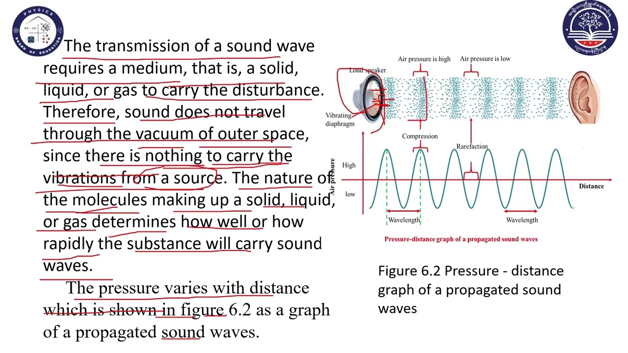














Underwater sound propagation is governed by fundamental physics principles including sound speed (approximately 1,500 m/s in water, compared to 340 m/s in air), absorption (about 20 dB/km in water), and refraction caused by variations in temperature, salinity, and pressure; these factors determine how sound travels through the ocean, with deep water creating a sound channel that traps low-frequency sounds for hundreds or thousands of kilometers, while shallow water environments involve complex interactions between sound waves and boundaries like the seafloor and surface, affecting detection range and receiver performance.
Physics of Underwater Sound: Sound Propagation & Acoustic Telemetry
Added:Basic wave mechanics, including concepts of frequency, wavelength, amplitude, and wave velocity.
The physical properties of sound propagation, specifically how pressure waves travel through different media.
Fundamental wave phenomena such as reflection, refraction, absorption, and the concept of attenuation.
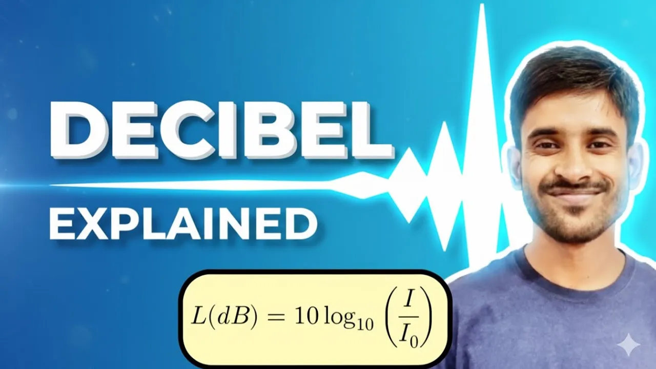
An understanding of the logarithmic decibel (dB) scale used to measure sound intensity and loss.
Design principles of active and passive SONAR (Sound Navigation and Ranging) systems.
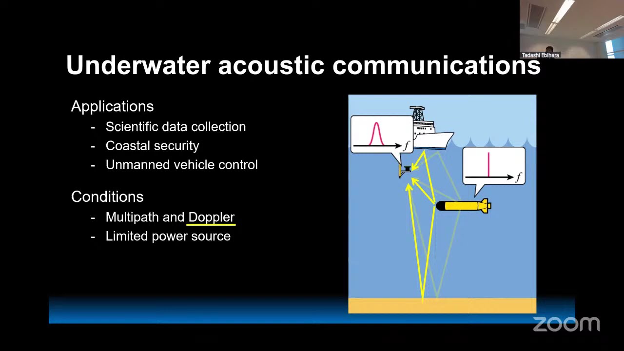
Underwater communication protocols, including modulation techniques for acoustic modems to overcome multipath interference.
Ocean Acoustic Tomography, using sound speed measurements to monitor global ocean temperatures and currents.
Marine bioacoustics, focusing on animal echolocation and the environmental impact of anthropogenic ocean noise.
13.6K views211likes31:56Original Release: 2020-06-26
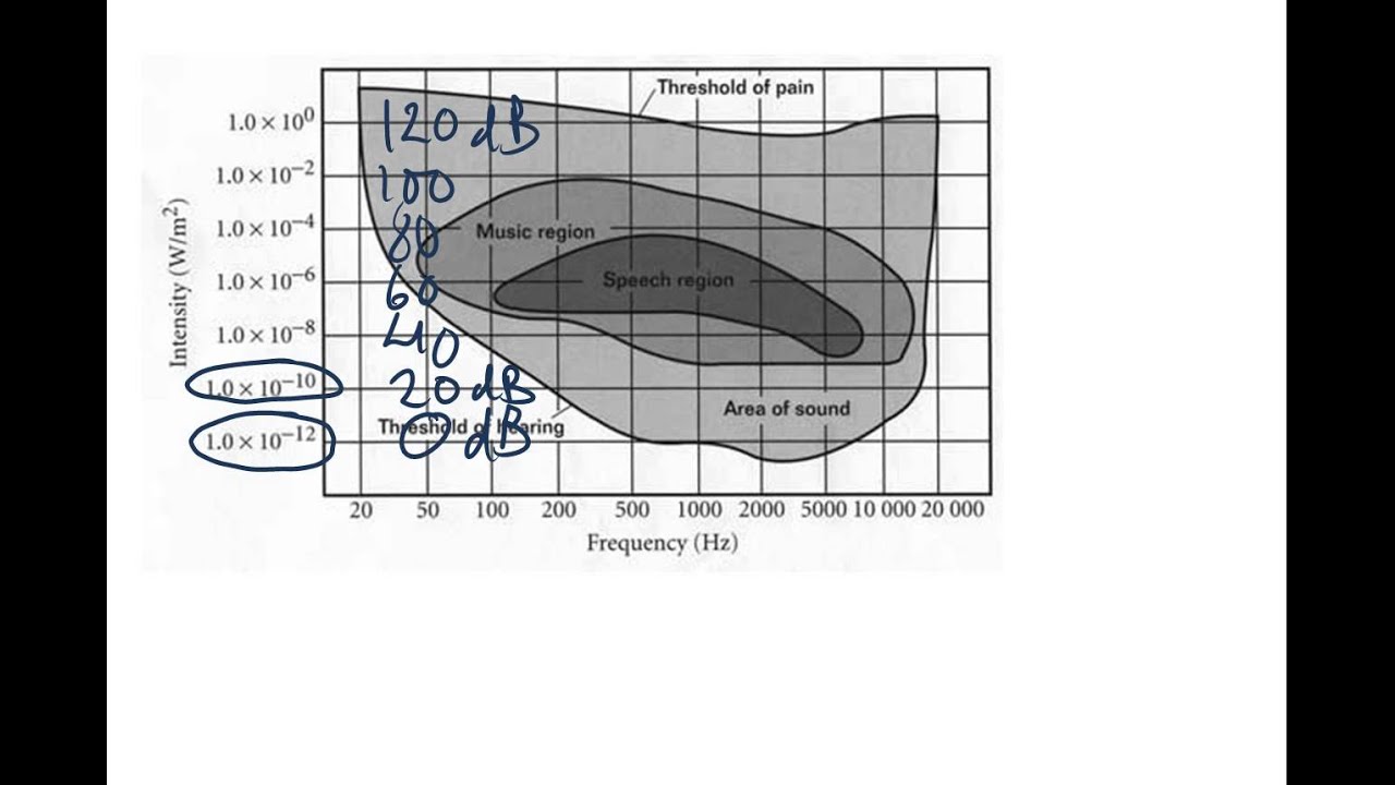
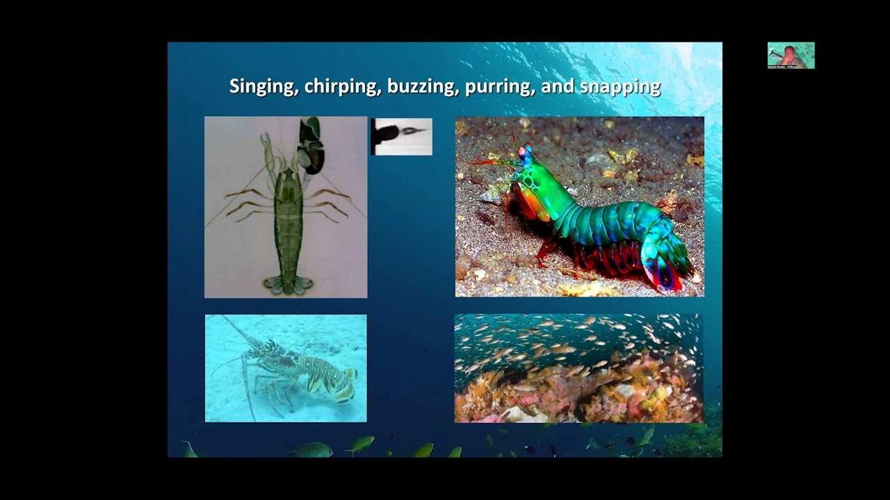
a panel event so now we're switching gears and we're going to talk about the physics of underwater sound and I remember at the ice EFT last year having some conversations with Michelle VOIPo especially and she's very passionate about the fact that you know these this technology that everybody here uses it operates with under it operates with sound underwater and so we really need to understand what factors can be influencing it and I thought oh my gosh you're right I need to know how sound X underwater I haven't take two taken physics since high school I should probably learn about this so talking to John PI he said I know the perfect guy who could give a lecture on this and he talked about David Berkeley David Barclay is a crc chair Peace Studies sound and sound propagation in lots of lots of different water environments but especially in deep water right yeah and he's actually writing a paper on this specifically so he's currently writing a paper about how sound can affect acoustic telemetry and so he's going to talk for the next 30 30 minutes about about the physics of underwater sound so thank you so much David okay great well luckily most of the physics of underwater sound is is high school-level I'm serious it's we're gonna talk about some really simple stuff here and but can have a really profound impact on how the performance of your of your receivers your fish tag receivers so the outline just a quick shortage talk very basic question what is sound and we'll talk about this yeah these concepts that are familiar to all wave propagation optics electromagnetic surface waves in the ocean right and then I'll talk quickly about the sonar equation and then a little bit of a study just a modeling study coming from the complete other end no experience in the field what can we do from physics up to predicting the detection range and performance of receivers and specifically the Halifax line receivers okay so first question got to ask go to start with what is sound and you know basically it's molecules crashing into each other denser rare for acting less dense and that communicates some signal that signal propagates with some speed right so the speed of sound and the amazing thing that that in in a dense material like water that's a nearly lossless signal so you nearly lost this process right so it can travel very far distance and the speed of which the signal goes depends on the properties of the material itself okay so like I said there's similarities between all these wave propagation phenomena so I have a question for you all why is the ocean blue why does it look blue not sound electromagnetic optics why does it look blue Oh in the back there absorbs every color but blue yeah exactly so this is the absorption coefficient this is a log scale here so the lower on this scale the less Banerjee's absorbs the optical energy and the higher the more it is and you can see this little rainbow here is that that's the optical spectrum the part of frequency spectrum that we can actually see with their eyes and blue is the least absorbed so that's why the ocean looks blue okay so we can ask the same question with sound and this is the same figure here with sound here you have frequency going from very very low frequency up to high frequency I put some things to orient yourselves here your baleen whales so the low-low calls you've got the piano keyboard that's like the highest note in the piano keyboard the lowest note is up submarine submarine I have any gifts there's no gifts in this one nathan has a nice gift size that's Mike that's gonna get to a DCP here and then here's your vem KO fish tags 6:9 killer hunter aiding kill Urtz and so you can just look on this figure and say okay obviously we should be using fish tags that are like 1 Hertz but that would you know the size of the speaker think of your subwoofer 1 Hertz is big right you need a huge speaker so if you want something small it's got to be high frequency the attenuation there are sort of the absorption so this is just the energy absorbed by the water itself there's about 20 DB per kilometer so the decibel the DB is just a relative measure and 6 DB means half the power so 20 DB or half half half and a little bit so you're a little more open than 1/8 of the power over one kilometer so that's why these detection ranges are so short now that's if he just had water and nothing else around and it was all just one isotropic perfect bath so that's the first thing to know and I should say that depends on temperature salinity pH bunch of things speed of sound the other thing so I said you know that the the speed at which that signal propagates has to do with the properties of the media so an air it's about 330 meters second - depends heavily on temperature and in water it's about five times that and in very dense things it's very very fast right so yeah there's some kind of intuitive physics in there that you should consider and really there's some great examples that where we experience all the time that that involved this these changes in density these changes in temperature that can manipulate the way of sound yeah so here's the classic one you want to go camping for the weekend you find a nice quiet lake and you're over here camping and there's some Kulik usually known as Yahoo's blasting the stereo cost the lake and you're like why can I hear all the way across this lake so well and well it's just idea of refraction right so you have the cold lake it's making this cold slow layer of air here and there's a warm layer where the sound travels faster up there and so what happens is the sound rays come up and they curve back towards you you can hear like super far away it's can be really really incredible right sometimes even get rays that are sort of bouncing along bouncing along that's why you can hear that conversation all the way across the lake so keep in mind yeah refraction again high school physics right but a good thing to keep in mind when you're looking at the ocean okay so here's the canonical deep ocean here here you have your monk Sound speed profile so you have warm warm salt warm fresh or warm salty water at the top as you go down the temperature slows the sound speed down then as you go down even further the pressure speeds that sounds to beat it back up again so you get this kind of sound speed profile that looks a little bit like a lens okay and for your sound source generated at the surface you can have raised that get trapped around this minimum this kind of sound channel axis it's called right so you can get basically sound rays that are propagating very very far distances you can get rays that are trapped in a surface duct that are prop that are bouncing off the surface of the ocean and all because of this refraction and this is a super powerful thing right so you can have a low frequency sounds where that absorption is super super low right you can ship or a whale or submarine generating sound gets into that san channel access and it can travel hundreds thousands of kilometers and so here's just the historical interlude this is the world's forum greatest living oceanographer he just died last year Walter monk he did this amazing experiment where they went up to hurt Island here they let off a couple of tons of dynamite or something like that and they could hear it all the way in Bermuda and up actually around on the on the west coast as well and so it was all just this idea of putting sound into that deep sound channel access and essentially go on forever now obviously when you start putting boundaries in there it become important so we have refraction we had absorption we'll just have to think about reflection right so here's a shallow water environment you have a source at the at the at the surface there it's bouncing off the bottom it's bouncing off surface and you want to understand well how will that impact the transmission loss or how much energy is lost every time it goes out in some range and so the question is what what governs the physics of the reflection of a sound wave at an interface and the simplest answer is just acoustic impedance so the impedance you may also remember from high school electronics okay density and Sound speed so there's a analogy to how current flows through a resistor but the idea that it's the product of the density in the Sound speed of a material so for instance at the surface right you have very very low density right the density of air is very low compared to the density of water and so essentially the impedance is like zero so you get a perfect reflector at the surface so if you had a perfectly flat surface of the ocean and you looked at it with sound it would look like a mirror your your Ray's would bounce off without losing energy any energy in the seabed on the other hand you can have a very hard bottom which is very you know high density high Sound speed we reflective a soft bottom which be kind of an equivalent density to seawater right a mud this can be sort of a almost the same thousand kilograms per meter cubed and so you can it can be more absorbent it can basically be acoustically transparent transparent the energy can propagate into the bottom and you won't get much of a reflection and so all these things depend on what might be at your study site the the sediment properties grain sides porosity density now the other thing of course is that I've drawn these as perfectly flat surfaces you can get a windy day and start to get some really rough surfaces up there you know that this and that can really impact how things reflect off the surface you can really you can imagine this ray is it a bouncing off perfectly flat surface there's a little wave there and it scatters it and so it can be quite complicated considering all of these things so those are all the very basic wave propagation things to consider now I just want to put this in here this is just to show you that even with these this basic knowledge you can do some pretty interesting research so this is a study we did recently and what we what we did is we put two hydrophones here in a muddy sediment we had an elastic basement an elastic muddy sediment and we listened to the noise so the sound of breaking waves was reflecting off the assessment we came up with statistical model and whoops and the basic idea was that just by listening we could compare the noise in this waveguide and figure out what all of these parameters so the compressional wave speed the sheer speed the attenuation so we could just listen and understand what the ocean was made out of basically what the seabed is made out of similar to you can imagine you're in a room and you can figure out if it's concrete walls vast walls or has carpet or whatever just by listening races do the similar similar type of stuff in the ocean I'm using this super basic physics so one last thing we need to consider is geometric spreading loss again something you might remember from high school and the basic idea is that if you have a source that's emanating some sort of energy let's say it be optical could be acoustical as the way propagate outwards you have to cover more and more surface area right four PI R squared in the case of just up limitless infinite media that you're working in and energy loss goes as R squared and so decibels are are a measure of relative energy so this is why there's such a convenient unit for a convenient unit to use and so basically the loss if the energy loss goes is R squared the loss in decibels goes as R squared the log you take it out 20 log R right remember that okay and for a cylinder so here have this sort of shallow water so now you imagine that your environments like a you know very it's trapped between two boundaries and imagining of perfect reflectors on either boundary now your energies are just propagating out like a cylinder and so the area now is 2h PI R energy loss goes down as R so now there's no exponent to take out you just have 10 log R DB right so these are super simple models to write away get a handle okay what you know if I had a tag in a ocean with no boundaries and no absorption this would be a really nice model to work with ok that's it that's all you got to know to understand transmission loss so it's very basic ok now I have another historical interlude I want to talk about putting sound in the ocean so you're actually putting sound in the ocean and this interesting fact the first person to ever make an underwater speaker was a Canadian Reginald Fessenden and it was actually used they would put these big low frequency sound sources so again this is like probably around ten to a hundred Hertz so that's you can imagine that a little impractical tag a fish with that and Mariners would actually go in the halls of the ships on foggy days and listen for the sound sources to guide the ships in when they couldn't see anything so this was like an interesting idea at the time but I have a question for you what great world event happened that brought much fame and fortune to original president and this technology happened the year after anybody anybody not war sight anok yeah because he figured out that not only could you hear you could you could listen for the sound but you can actually make the sound it could send it out it would reflect off of something like to say the seat but seabed or an iceberg and it would come back and if you hear that reflection you go now there's an iceberg there be careful and he suggested we put it on these ships and yeah it really helps push the thing for it now of course then then the war the war as well they figured out oh it also reflects off submarines and that that was a whole other thing and that's we came up with these simple equations known as the sonar equation so there's a whole family of these types of engines and again because you're using the bull decibels it's all a relative measure and their log right so log a times B is log a plus log B you can do simple things like this ok the signal-to-noise ratio so the amount of signal above the noise level that I'm receiving is equal to the source level minus the transmission loss that's all the stuff we just talked about - the noise level so there's some background noise level let's say in the ocean and so this is your you know super simple model and with no fish tank experience the complete opposite of Nathan this is where you're gonna start well what is going to be detection ring and the detector yeah the detection range and maybe the detection efficiency of my receiving system and so I put a little asterisk here the one thing we actually need to know this is so this is signal to noise level that's if you just had say a microphone and you recorded it you would say here's the noise the signal bumps up that ratio between the two things that doesn't necessarily mean that your algorithm that's onboard your receiver that makes a detection is gonna work it might meet you know it might need me to speak really loud I might need a double the signal-to-noise level then say you might need when you're visually looking at the data so there's there's a certain bit of information that's missing here but this is as close to a model that we can get to do these predictions so if we dissect these terms a little more a little more completely so the source level well that might depend I read tag I don't really know I'm not the manufacturer and the coupling with seawater there's actually when they talked about the tag if it's right next to swim bladder you know you're gonna have reflections off the the swim bladder or it might not be very well coupled to the body or who knows what right there could be the fish has weird lumps but it's gonna it's gonna differ it's gonna differ there's some physics there that's really important for the transmission loss well we talked about source so the source receiver position so that in range in depth that's gonna be very important the bathymetry the shape of the Basim 'try right the sediment type so how reflective that mysterious the sound speed depth profile so whether it's refracting upward downward you know what what's happening there and you know all of these all of these things really matter and the position your source and receiver next to those boundaries can be very important if you're far away from the boundaries they don't matter if you're close to the boundaries that do matter most of the time these receive a lot of mountain so the boundaries do matter for the noise level a little bit trickier so we're up in pretty high frequency in kind of conventional wisdom would say that mostly just have wind wave toys so we heard about that last talk and maybe some rain generated noise rain you know makes a little entrains little air bubbles every time you have a droplet fall it's very very noisy it's like when you're in a you know under a tin roof and hear the rain banging way up there in the ocean it's the same thing you might have thermal and electronic noise so noise on your Apple sensor is on your electronics that you might not be able to well-characterized and I put here the analog-to-digital saturation from flow noise or ship notes so ship noise is very low low frequency and flow noise is also very low low frequency but sometimes it's so energetic that it saturates your recording system and you're not able to record high frequency noise so like in riverine systems I could see this being a huge a huge problem and so then and then the last thing here is SNR we have this question how much is needed for positive section is a 0 DB 3 DB 6 DB 20 DB kind of hard to tell so with all that with that simple modeling framework I'm just gonna give a little study that I've been working on for the last little while trying to understand if we can predict the performance of these these receiving systems and so the study site that I'm using here is that line it's a whole bunch of stations as a whole whack load of data and they're into kind of they're in a very the environment varied you're going from like super littoral off to the shelf break so I'd imagine there's some different oceanography that's going to come into play there's some different symmetry that's gonna be important I just use uniform bottom properties here to kind of take that out of the equation but also just don't really have the most data on on what that is but I used a whole bunch of Sound speed profiles so these are depth Sound speed here in the x-axis and they're these black lines are tracks from gliders I just collected them all in every around one station I drew a circle these are all the ones that were collector around that sir and I simplify them to some representative sounds profiles and then used what's known as ray tracing program so you can calculate transmission loss using a computer program at high frequency and this is one called bellhop and each one of these represents range and the x-axis and depth on the y-axis the white line is the FEMA tree and the intent the color intensity is the transmission loss so the darker started the darker the color of the higher actually sorry the color intensity is the intensity of sound so now this is where your source is it's quite bright send some sound out and then as it gets further and further away it gets less and less intense and you can see that the sound speed profile these are three different sound speed profiles really impacts the shape of how the rays propagate and then I did that at each station looking in different different directions and you can see that as you go around in Direction this is some detection probability statistic the it changes because of the asymmetry slightly changing and stuff like that this is small changes and I was kind of curious to see well how how much would they impact our ability to estimate the detection range for the noise is a little trickier these are some classic curves the wentz curves so I was really just estimating or assuming here at 69 kill Urtz that we just had wind-driven wave breaking noise not always the case there's biological noise there's other sources of noise that might come into play here but making the simple assumption now that noise you can read the number off of here right you can choose a wind speed read a number off of here and put that as your noise level term but actually there's some spatial spatial differences to how that noise is distributed in the water column right and so what we did is we did similar a modeling thing where we put noise sources all surface and thumbed over we assumed that there was breaking waves we summed over all of those that would give us the noise source at like say 100 meters 150 meters depth or whatever so we came up with a little simple physical model and that turned out to be pretty important when you sort the stations by depth so this is the stations in geographical order and then the noise level in DB if you assume the wind is 25 knots okay and so this empirically the source levels empirically determined from previous data but it's relative magnitude according to the station position was computed in law small there are little noise model and so when you sort them by a geographical order you don't really see any that meaningful there but here I've sorted them by station depth and you can see that as the station gets deeper the noise level increases this is a similar type plot now here what I have is the detection range for a 95% detection efficiency as a function of Sound speed profile so each one of these is a different one of those Sound speed profiles that I extracted near the station and just ran the computation and the overall the different directions and then computed the mean and then these whisker box and whisker plots or whatever these are called a very popular in biology we don't use them in fits very hot but I have to say um and so you can see the huge amount of variability here right so you choose this pre profile your detection range with art are under our model assumptions could be 500 meters and or it could be 750 meters so in terms of volume right think about detection volume that's really what you need to know right if you're trying to understand your sample space that's it that's a huge amount right so we took the station means and then here I have them bought at a geographical order here across the shelf break again no real trend but a very significant you know basically a factor of two at some stations in terms of their detection range but when you sort these stations by depth you get a more full system so here's detection range as a function of station depth for 95 percent detection 50 percent detection efficiency which is just to say this will this is predicting 95 percent of the time you're going to hear the tag and this is predicting 50 percent of the time you're going to hear the tag and you can see that that depth effect from this is is very significant I plot for comparison I plotted those against this is this was on the vehm co website this was their detection range as a function of wind speed they shared and I plotted here's the 95 percent detection line here in blue but there's a big caveat right so the detection radius depends on the station depth so here I just chose 100 meter station depth the wind speed so this is for all wind speeds and the required signal-to-noise ratio ratio that the algorithm needs to you know the hardware needs so many DB's above the background noise to make a positive detection that's totally unknown so essentially the caveat is that these lines can move up and down as much as much as you want with that unknown information but at the same time whether you know so this is this is the same data kind of presented in a different way here I have chosen 100-meter stationed depth I've chosen 25 knots of wind so that gives you a certain detection range and like I said you can kind of move this line up and down I was 0db signal-to-noise ratio required for a positive section if that number is 20 DB these lines are obviously going to move down but not this variability and so here's the true this is a true box and whisker plot I know for sure here and you can see that 30% increase intersection volume is is pretty significant if you're trying to understand like population density estimate that type of problem so from the last speaker of course absolute values required experimental verification calibration this is just a computer model for now but it would be really amazing to try and go out and and compare some of these results to some of these Sentinel studies that are that are actually carried out and to see to see how much variability can truly be there like I believe Nathan had that kecil paper up where there's a plot where one day the detector the detector efficiency is like 80% on a sentinel tag and the next day it's 20% and that could be just you know a thermal warming or some oceanographic thing happening and if you could predict those and account for them then it makes your data just that much more powerful so yeah some conclusions we started off basically with I want to say yeah high school physics was enough to get us to a pretty accurate transmission loss model and we need really we need those type of models to predict the time-dependent detection performance some of the conclusions so far that the receiver depth the background noise level injection algorithm they those determine the detection range and the ocean air oceanographic variability influences detection efficiency of tagged marine animals so that's working towards being able to predict that so that could be something in studies that could be accounted for and that's it if you have any questions yeah so the noise okay so the question is so you have a receiving system where you actually have an in situ measurement of background noise right and but that detection efficiency shows nor no correlation with right so I mean I suppose it could be the actual animals moving that are just driving your section efficiency right I mean that could be one solution oh the stationary reference text okay yeah I mean so it's kind of I'm kind of a little bit curious in terms of how the noise was measured this is this is reported by the instrument itself okay yeah okay because because one thing I have been considering is the stationarity of the noise right so if you have say snapping shrimp weight like you'd have I'd imagine down there say you take a 10 second window of data and you calculate the noise level from that that might be one way to estimate the noise but it is the noise stationary over ten seconds right if you have lots of snapping trip there'll be moments where the noise is very very very loud on the order of say tens to hundreds of milliseconds I guess and so that could cause an interference I guess the detection algorithm that would maybe be my first guess that why the noise level itself might not match up with but I don't know how it's calculated I'm not sure if that that's my hypothesis on the hotseat what do you think is that possible it's a hard it's a hard thing to do it's a hard thing to do because it you are like the tag the tag single itself is quite short and so you you're kind of in the realm where the statistics of stationarity break down so if you have something where you have a if you imagine your noise is a distant distribution you have something that has a very very heavy tail from snapping shrimp then kind of common assumptions are gonna just not work right so using that mean noise level is just not gonna give you a an accurate say yeah correlation just just an idea not sure if I'm right no that's fine that's it's super interesting topic yeah any other questions yeah I mean you have like short time scale processes like you know on a calm day sun shining down you get develop these like surface layers but then you have things like eddies spinning up from the from the Gulf Stream that's been up onto the shelf and bring in you know warm water with them or cold water so you yeah it's just it's a huge amount of physical processes that are happening out there yeah and as well as seasonality this is used I used profiles from the entire year as well so yeah I mean just depends who's asking it's always the question like so most of the work I do is like at a hundred to a thousand Earth's like low frequency stuff and pretty much you know if you went to the Navy and said how hey what's your detection range on a submarine they'll give you a number but most sonar operators would say that numbers plus or minus 10 dB basically there's not a there's not a huge amount of confidence in these models in general but working very hard to produce that and and working at higher frequency is somewhat less daunting because like you wouldn't really imagine that boundaries play much of a factor at these super high frequencies because you're not going far enough to scatter off the boundaries many times but right if we can get that one scatter off the bottom that one scatter off the surface nailed down pretty well then I think we could have a pretty good chance at these models being able to predict it's pretty well yeah why is the sky blue no one's gonna ask me that we did the ocean but okay
Up Next
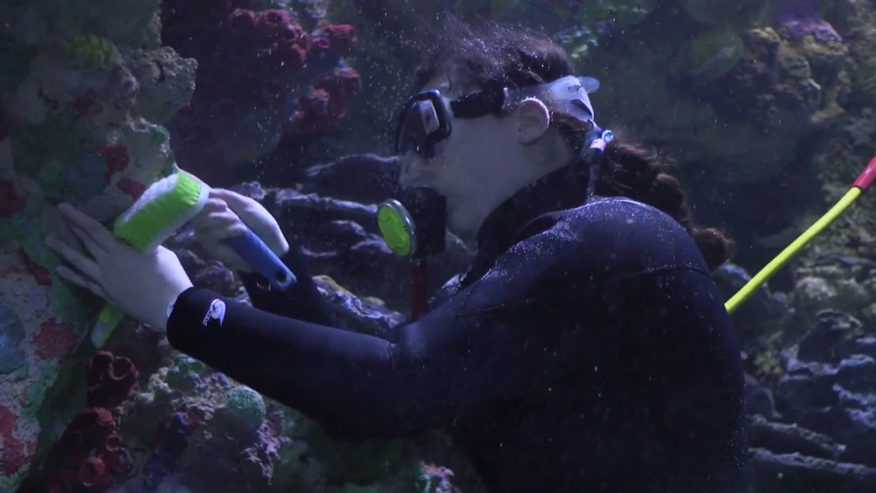
5:01
How Sound Travels Underwater | Physics & Marine Life
@discoveryworld
45.5K views•2020-05-27

12:53
21cm Hyperfine Transition in Neutral Hydrogen: Radio Astronomy Basics
@AaronRobertParsons
12.4K views•2011-10-13

32:32
NMR Spin Physics I: Zeeman Effect, Resonance Condition & Larmor Frequency
@nptel-indianinstituteofsci8064
2.3K views•2024-01-17

27:14
Entropy and the Second Law of Thermodynamics Explained
@veritasium
27.5M views•2023-07-01
Related Study Plans & Knowledge Roadmaps
Structured learning paths in Physics
physics
Nuclear Physics (Decay, Fission & Reactors)
01Atomic Structure and the Binding Force
02Radioactive Decay and Half-Life
03Nuclear Fission Mechanics and Chain Reactions
+ 2 more learning modules
12h5 modules
Explore Roadmap
physics
Soft Matter (Polymers, Colloids & Rheology)
01Foundations of Soft Matter & Thermal Forces
02Polymer Physics and Macromolecules
03Colloids, Surfactants, and Self-Assembly
+ 2 more learning modules
38h5 modules
Explore Roadmap
physics
Analytical Mechanics: Lagrangian & Hamiltonian
01Mathematical Foundations: Calculus of Variations
02From Newtonian Mechanics to Constraint Dynamics
03The Principle of Least Action & Lagrangian Mechanics
+ 3 more learning modules
28h6 modules
Explore Roadmap
physics
General Relativity (Spacetime & Cosmology)
01Foundations of Relativity: Special Relativity
02The Geometry of Spacetime: Equivalence Principle & Curvature
03Einstein's Field Equations: The Mathematics of Gravity
+ 2 more learning modules
55h5 modules
Explore Roadmap