





















Dynamic Light Scattering (DLS), also known as photon correlation spectroscopy or quasi elastic light scattering, is a non-invasive technique that measures particle size by detecting the rate of intensity fluctuations in scattered light caused by Brownian motion; smaller particles diffuse faster and produce rapid intensity fluctuations, while larger particles diffuse more slowly and produce slower fluctuations, allowing the hydrodynamic size (the diameter of a hard sphere diffusing at the same rate) to be calculated from the measured diffusion coefficient using the Stokes-Einstein equation.
Dynamic Light Scattering (DLS) for Particle Size Analysis Basics
Added:Basic wave optics and light scattering phenomena, particularly Rayleigh scattering, which explains how particles scatter incident light.
The physical concept of Brownian motion and how thermal energy drives the random movement of suspended particles.
The variables of the Stokes-Einstein equation, specifically how diffusion coefficient, temperature, and solvent viscosity relate to particle size.
Fundamental statistical concepts, particularly autocorrelation and how it is used to measure the similarity of a signal with itself over time.
Advanced mathematical models for DLS data interpretation, such as the Cumulants method and the CONTIN algorithm for polydisperse samples.
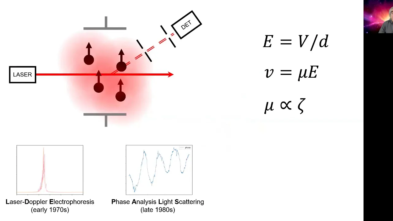
Electrophoretic Light Scattering (ELS) for measuring Zeta Potential to assess nanoparticle surface charge and colloidal stability.
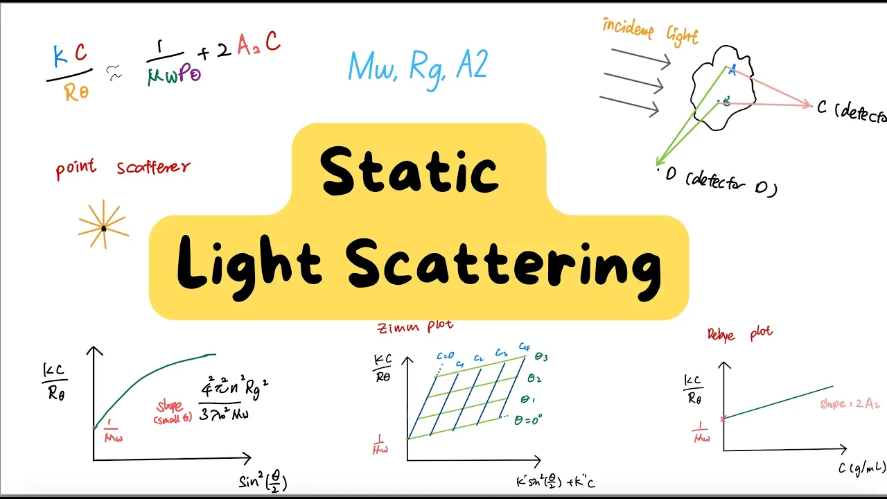
Static Light Scattering (SLS) techniques to determine absolute molecular weight and the radius of gyration (Rg).
Practical sample preparation protocols and troubleshooting, including managing dust contamination, concentration effects, and multiple scattering.
81.3K views910likes19:24Original Release: 2018-05-18
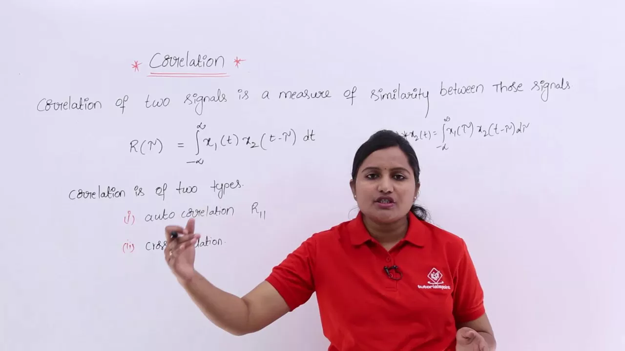
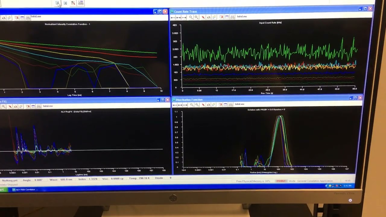
[Music] hello everyone thank you for joining us and welcome to today's presentation while we going to discussing a basic introduction to dynamic light scattering for particle size analysis it should probably take around 30 minutes and to take us through this presentation I'd like to introduce dr. Micah Shiva who is a Technical Support Manager and he has a PhD from the Polytechnic of Wales where he studied the physical biochemistry of lipids ohms using nuclear magnetic resonance techniques he followed this with a postdoctoral research into the concern on drug delivery at the University of Manchester now Michael joined us in 1996 as a product technical specialist a couple years later was appointed to his current role Larry's responsible for the product technical specialist and applications groups based in the UK so with that in mind I will now hand over and focal Mike thanks Craig welcome everybody and this talk is called dynamic light scattering in 30 minutes it's designed to be a quick short discussion really of the technique how the technique works and so on so those of you that use more than plan elliptical products will know that the Ziegler signs or series consists of three instruments so this talk today is really applicable to all three we've got the Nano they're the microfi and the APS so the basics of the technique are the same for all of these and instruments so this is the agenda three very short agenda I'm going to start by discussing Brownian motion and then going on to talk about correlation and finally how we analyze the correlation function how do we get size information out of the correlation function itself so let's start with Brownian motion so dynamic light scattering and I suppose the first thing I should say here is different people know this technique by different names we are going to refer to it as dynamic light scattering today sometimes it's known as photon correlation spectroscopy and sometimes it's known as quasi elastic light scattering and so the three different names for the same technique and the technique is non-invasive in other words we place our sample into a queue that we shine a laser into that sample the sample is not influenced at all by that laser so when we take the sample out of the instrument it's in exactly the same state as when we put it in so it's a non-invasive technique and it's capable of measuring the size of particles and molecules in suspension and what we're specifically looking at is Brownian motion and the important thing about Brownian motion it's a random movement so these particles and molecules are moving around randomly because they're constantly being bombarded by the solvent molecules that surround them and what dynamic light scattering does is to measure the speed at which these particles undergo this Brownian motion small particles diffuse rapidly large particles diffuse slowly the velocity of this Brownian motion is called the translational diffusion coefficient this is given a symbol D now we provide diffusion coefficient information within our software but the majority of your users would much prefer talking about particle size so the way in which the diffusion coefficients have converted into size is through the Stokes line just an equation that you can see on this slide so what we end up with is a hydrogen and a Gradius we know Boltzmann's constant we know the temperature at which the measurement is made at and therefore we know the discus 'ti of that sample we know pi and therefore from this measured diffusion coefficient we can get our particle size or our hydrodynamic size what do we mean by hydrodynamics size it's simply the diameter of a hard sphere that diffuses at the same speed as the particle and molecule being measured and this is going to be dependent on various things firstly ionic strength so ionic strength that's going to influence the thickness of the cloud of ions that exists around the particles so those of you that have done any colloidal chemistry will know about something called the Debye length the Debye length is the thickness of the electrical double layer the cloud of ions that exists around the surface of the particle and molecule and that's inversely proportional to ionic strength so as we increase on expense we compress the Debye length and therefore the size we get from dynamic light scattering for any particle suspended in a salt solution is going to be it's smaller than the size we would get to the same particle if it was suspended in deionized water for example surface structure can influence hydrodynamic diameter because if we've got let's say nodes or polymer layer on that surface if the adsorbed polymer layer has a conformation in which the molecules are sitting out into the medium then that's going to influence the diffusion speed and then we have shape if we have irregular shaped particles as it undergoes random diffusion and during the course of a measurement we are going to measure different diffusion coefficients depending on which orientation the particles are in remember that the size that we get from the technique is the diameter of a sphere which has the same average diffusion speed as the particle the molecule being measured so that's what cement when we talk about hydrodynamic size so what is a DLS instrument consists of well I mentioned earlier that what we do is we take a suitable cuvette which we got here we put our sample into that key that the cue that could be plastic disposable it could be glass it could be quartz we've got low volumes cuvettes for instance we can measure down as low as 2 microliters in volume we Casso a laser into that sample and the particles or the molecules in there will scatter light at all angles now in this particular schematic we we are detecting the light here at a 90 degree angle to the laser beam for the majority of instruments that we currently sell the vast majority will measure at an angle of 173 degrees to the beam and we call this and back scatter detection now the detector that we use is capable of counting individual photons it's a photon counting device the detector that we using them as an avalanche photodiodes so it's very sensitive and basically what this detector the signal it produces is simply the number of photons detected as a function of time now you'll see in this little schematic here the intensity is fluctuating over time the important point to make is that the time scales over which we're observing this scattering intensity are very rapid we're talking nanosecond microsecond millisecond time scales if we observed the intensity of a much longer time scale second tens of seconds we wouldn't see these fluctuations the intensity would be pretty much average so this signal is then passed into it's all signal processor and the processor that we use is called a correlator and you can see why some people know this technique as photon correlation spectroscopy because we are correlating the detected photons I normally represent the correlator as a dark gray box as you can see because for the majority of people that use dynamic light scattering instrumentation they don't really understand what goes on in that correlator but ultimately that's the heart of the instruments the heart of the technique so it's important to try and have an appreciation of what correlation is now if we were to look at the intensity fluctuations from a sample containing very small particles nanoparticles or molecular solutions we would find the intensity fluctuates very rapidly conversely if we've got much larger particles hundreds of nanometers or microns in size because their diffusion speed is much slower the intensity fluctuates over much longer timescales so the important message here is that the rate of fluctuation in the scattering intensity is determined by the size of the particles and that's really the basis of the technique now the question is well why does the intensity fluctuate so here's a schematic which tries to explain that let's imagine we've got two stationary particles and we pass a laser across them they might scatter light as you can see at the top of this slide where we have got a maximum in one opposite a maximum in the other or a minimum in one opposite a minimum in the other now in that configuration we have what is known as constructive interference so when those scattered beams of light arrive in our detector we get enhanced intensity if however the position of one now moves with respect to the other so we're now looking at the bottom half of the slide we've now got a configuration where a maximum in one is obviously a minimum in the other conversely a minimum in one's opposite a maximum in the other and in this configuration we have complete destructive interference and when they arrive and exactly the resultant intensity is now zero and they effectively cancel each other out now these are the two extremes that we could consider we could have completely constructive interference or completely destructive interference now when we take a measurement in a DLS instrument we're not talking about two particles or two molecules which are stationary we are measuring billions and they are all undergoing random diffusion so their position with respect to the detector is constantly changing and as a result of that we have an average intensity being detected and that average intensity fluctuates over very short timescales and that really is the basis now of the BLS technique now we go on to talk about correlation because that's all well and good we can detect these fluctuating intensity signals how do we analyze them well we come to correlation and what correlation is is a technique for extracting the time dependence of a signal in the presence of noise and this time analysis is what's carried out by the correlator now there are not many equations in this presentation but this one is fairly straightforward what the correlator does is to construct the time autocorrelation function which is given a symbol of G of the scattered intensity and this happens according to this equation now when you look at this equation what we have got here so we are going to observe the scattering intensity at time zero we are then going to multiply it by the scattering intensity at time zero plus a delay time and I'll mention what that what I mean by delay time shortly and then we're going to divide it by the intensity at time infinity squared now time infinity sounds a very long way away but in reality we're talking a couple of seconds because the diffusion processes that we observe in dynamic like scheduling occur over microseconds millisecond timescale so if we look at this signal over a couple of seconds in time we are really at infinity and so the correlator continuously does this process of multiplying numbers of photons together separated by a delay time and the correlator has a number of delay times associated with it and these delay times start in the nanosecond time range they go all the way through microsecond millisecond and that's a seconds so we are we're basically covering about 11 decades of time in our correlator to try and understand that is a schematic so let's imagine this top trace is the intensity fluctuations that we've detected from the sample containing very small nano particles or a sample of molecules in solution proteins or something like that the intense is fluctuating very rapidly the bottom trace is from a sample containing much larger particles so because of the diffusion speed is much slower the intensity fluctuates now of a much longer time scales so what we're now going to do is we're going to make copies of the signals and we're going to place the copies on top of the original signals and what we can say is at time 0 the the copy of the signal is absolutely identical to the original signal so at time 0 the signal and the copy of the signal are perfectly correlated now perfect correlations given a value of 1 and as you can see on this y-axis here we've got a value of 1 up there if there is no correlation in the signal then obviously we've got a value 0 down here now what you will notice is in this case we have an intercept which is not actually at a value of 1 and I deliberately done that simply because it's impossible as instrument manufacturers to develop an instrument which contained no lines there is going to be noise within the system what we try to do as the manufacturer is to minimize that noise as much as we can and that comes down to the quality of the components that we use the laser that we use the detector that we use the optical configuration the optical components that we use we're trying to minimize this noise as much as we can those of you that have got backscatter nanos to nano ash nanos their des known as LSP for instance in backscattered typically we would expect intersex should be above point 9 so we can express that as a percentage that's 90% usable signal that's pretty impressive Craig mentioned I started here in 1996 well if we were getting intersex greater than about point four they were amazing I mean today if we had an intercept as low as that would say there was a major problem so put it into context we would expect very high intercepts now from the optical configuration that were using what we're now going to do is we're going to shift the signal with respect to when we started so now we've introduced our first delay time in our correlator those of you that are nano users the first delay time that we use in our correlator is 500 nanoseconds okay so after 500 nanoseconds in the top signal here because this is fluctuating very rapidly there is a significant loss in correlation over a very short period of time however in the bottom signal because that's taking much longer to fluctuate yes it's lost correlation but it's lost correlation not to the same extent as the top one if we now go on to the second delay time and again in the Nano the second delay time we use is a thousand nanoseconds which is one microsecond we see that the correlation has decayed once more in the top signal here it's decayed much more rapidly than it has in the bottom signal and again just to reiterate the reason for this more rapid loss in correlation in the upper signal is because the thing with itself is changing more rapidly with time now we can keep on doing this so this this is now what the loss of correlation looks like after the third delay time until eventually we get to infinity and at infinity the signal bears no resemblance to when we started so we've now reached a correlation coefficient here of one sorry it's zero there's no more correlation less in the signal now an important thing to say is for any random signal and of course this signal should be random if we were observing it from particles and they're doing Brownian motion there should be no ordered processes going on in there if it's a random signal the loss of correlation is an exponential process and what you can see there on the right-hand side of this slide we have got these exponential decay rates in correlation as a function of delay time now you'll notice that currently this x-axis has a linear scale so we have a classic what we would call classic exponential decay curve now if we plotted that exponential decay on a logarithmic x-axis what we would see is what we get out of a measurement so this fundamentally is what we get from a DLS measurement we call this the correlation function or correlogram or autocorrelation function and what we're observing here on the y-axis is the correlation coefficient the similarity of the signal with respect to itself plotted as a function of delay time and you can now see on this axis we are covering a wide range of delay times we're starting at 500 nanoseconds or half of microsecond and we're going all the way up to a couple of seconds in delay time in this upper signal we can see that this loss in correlation is occurring over quite short delay times typically in this example over a few microseconds in the bottom signal however the correlation persists for longer and we don't really start to see a loss in correlation until we're up to a few hundred microseconds in this example
Up Next
42:19
Quantifying RNA Encapsulation in LNPs Using the Modified RiboGreen Assay
@PrecisionNanoSystems
13.3K views•2020-06-27

12:54
Triumph of Orthodoxy Icon: Byzantine Art & History Explained
@BenCallan
2.1K views•2024-08-06

3:45
Isothermal Titration Calorimetry: Binding Affinity, Enthalpy, Stoichiometry Explained
@MalvernPanalytical
108.9K views•2014-07-22

1:42
Game of Thrones Opening Credits: A Cinematic Analysis
@gameofthrones
46.3M views•2011-04-18
Related Study Plans & Knowledge Roadmaps
Structured learning paths in General & Interdisciplinary Studies
general-studies
Elevator Engineering: History, Physics & Cities
01From Hoists to Safety Brakes: The Dawn of Vertical Lift
02Hydraulic vs. Traction: The Engineering Physics of Elevators
03Modern Speed, Safety, and Algorithms
+ 2 more learning modules
12h5 modules
Explore Roadmap
general-studies
Rubber: Material Science, History & Geopolitics
01Origins of Natural Rubber & Mesoamerican History
02The Chemistry of Natural Rubber & Vulcanization
03The Geopolitics of the Rubber Boom & Colonization
+ 2 more learning modules
12h5 modules
Explore Roadmap
general-studies
Containerization: Evolution, Logistics & Trade
01Ancient Trade & Bulk Cargo: Amphorae to Barrels
02The Industrial Revolution & Cardboard Packaging
03The Containerization Revolution: Malcom McLean
+ 2 more learning modules
12h5 modules
Explore Roadmap
general-studies
Textile Tech: Evolution, Labor & Global Impact
01Pre-Industrial Textiles: Handloom & Cottage Industry
02Mechanization: The Spinning Jenny to the Power Loom
03The Factory System & Global Labor Transformation
+ 2 more learning modules
10h5 modules
Explore Roadmap