











![Lesson 5-3 [Data Management and Analytics] Multi-Sensor Data Fusion](https://i.ytimg.com/vi_webp/Zyq7_jhhCGU/maxresdefault.webp)
![[3D-DLAD-v4] Strategies and methods for automotive sensor fusion, Robert Laganiere](https://i.ytimg.com/vi/iSAU3plRnJk/maxresdefault.jpg)






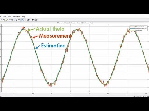
The Kalman Filter is a recursive algorithm that estimates the true state of a dynamic system by combining predictions from a mathematical model with noisy sensor measurements; it works by first predicting the next state based on previous estimates and control inputs (using linear system equations), then correcting this prediction using actual sensor data through a weighted combination determined by the Kalman gain, which optimally balances the confidence in predictions versus measurements to produce an improved state estimate.
Kalman Filter Tutorial: MATLAB Implementation with Bayesian NINJAS
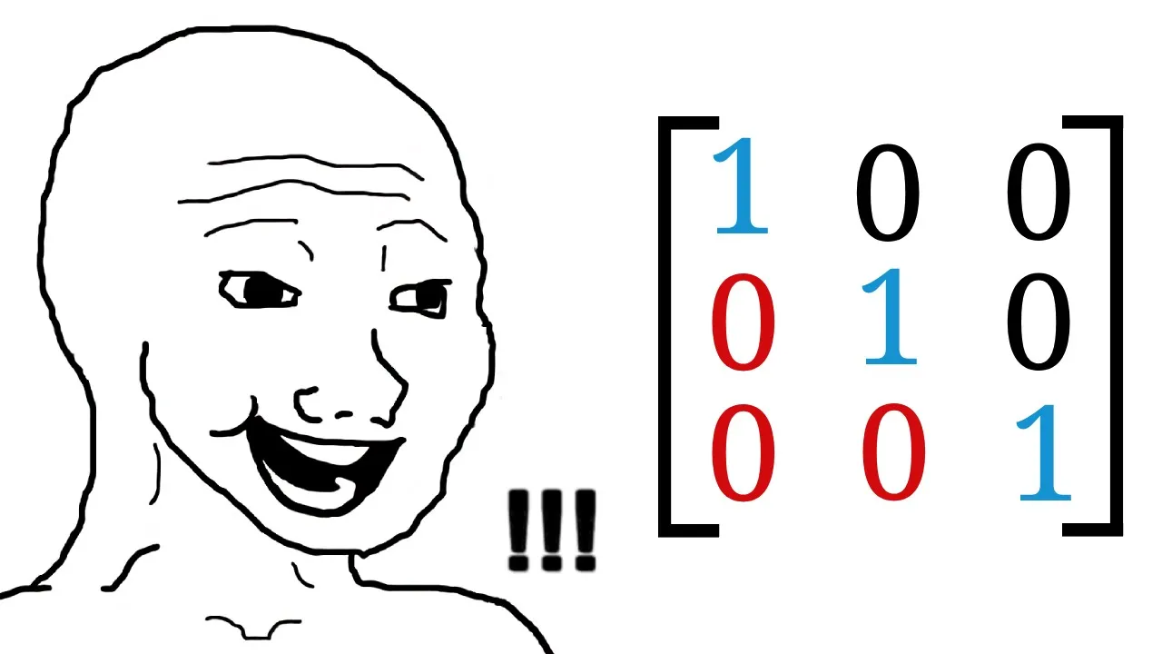
Added:Fundamentals of Linear Algebra: Understanding matrix operations, vectors, and state-space representations of dynamic systems.
Basic Probability and Statistics: Familiarity with Gaussian (Normal) distributions, mean, variance, and covariance matrices.
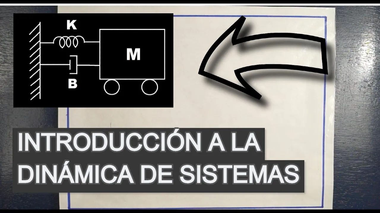
Introduction to System Dynamics: Concepts of state transition, process noise, and measurement noise in linear systems.
Basic MATLAB Programming: Ability to write scripts, manipulate matrices, and plot data in MATLAB.
Nonlinear State Estimation: Studying the Extended Kalman Filter (EKF) and Unscented Kalman Filter (UKF) for non-linear system dynamics.
Advanced Sensor Fusion Techniques: Integrating multi-sensor systems (e.g., IMU, GPS, and LiDAR) for autonomous vehicle navigation.
Particle Filtering: Exploring sequential Monte Carlo methods for state estimation in non-Gaussian and highly non-linear environments.
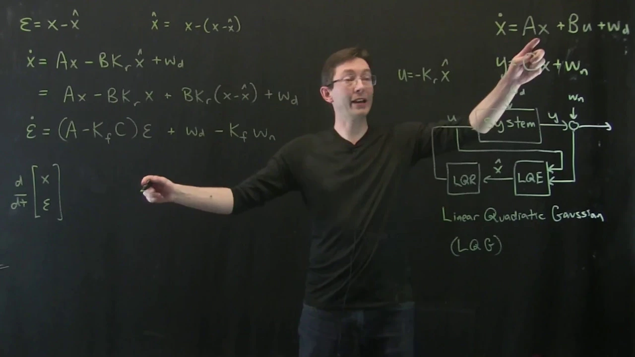
Linear Quadratic Gaussian (LQG) Control: Combining Kalman filtering with Linear Quadratic Regulators (LQR) for optimal feedback control.
380K views2.2Klikes9:29Original Release: 2011-04-26
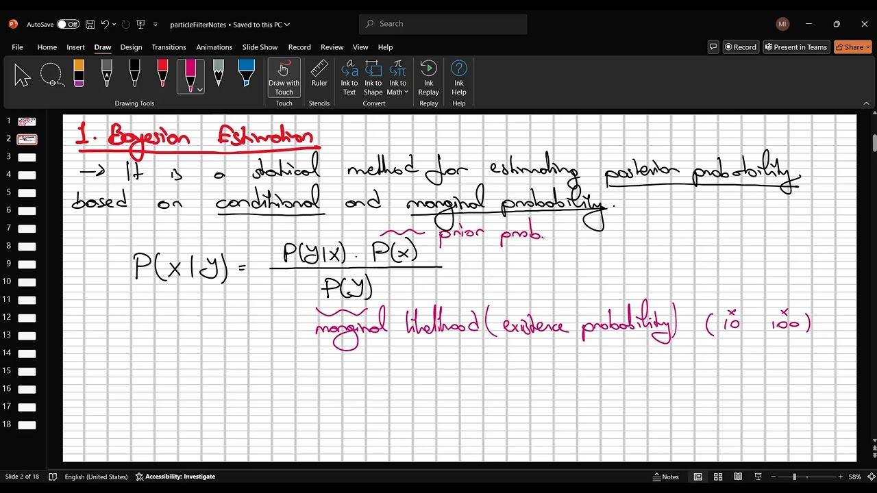
hello and welcome to the latest episode of student Dave yay okay today we're going to talk about the almighty common filter yeah everyone loves the common filter computer scientists engineers neuroscientists elves everyone loves a common filter why cuz it's incredibly useful um no okay well we'll talk about exactly what the common filter is its implementation in in a kind of like a general sense then we'll talk about a specific example going back to our beiji ninja hunting Quail uh and their issues with quail and then we'll do a mat lab implementation of that so you kind of see the whole package like you did for the recursive basan filter okay so what is the common filter well before we talk about that let's just recap with the curs what the recursive Beijing filter is because this is kind of founded on that you can the the common filter is kind of an example or a specific case of the beijan filter so again the beijan filter we go go back to the old videos if you want but uh I'll just give a little recap it's a probability of hypothesis given the data equals a probability of hypothesis times the likelihood of the data given the hypothesis all over the probability of the data right and so what we did is we took our hypothesis our posterior brought that back as a prior and reiterated iterated iterated rinse and repeat until our shirt is very clean or until our state uh estimation is as good as we need it so more generally what is this this is is saying the probability of a hypothesis at time T given the hypothesis at T minus1 and the data at T right that that that's really what we're doing right but this is kind of constraining our state estimate or our states or the things that can happen cuz basically we're holding the state constant the state isn't moving and we're just kind of estima as we get more and more data from it but what if what if we want to model something more complex so let's look at an example say we have a robot a a trash can robot do robot goes around picking up trash and you it's got a little body there's his head it's got like a little alien head and it's got ears and we're going to give this a name WALL-E the why don't you can't sue me Disney Wall-E okay so there he is and he's off in the desert and his job is to pick up trash he's a trash machine okay and so he's going around picking up trash and what he needs to know is he needs to know where he is other than how to pick up trash he needs to know where he is so he's got GPS in him right and just like all GPS like you have in your smartphone it can be really dumb and full of error right so let's say this is the probability of where we think we are and here's the robot and the robot think he's right here right now okay then the robot's going to move he's going to turn on his Motors and go somewhere else let's say he wants to go to this position over here well he can figure that out just from the command he sends out right I mean he commands his wheels to move so he could tell figure out wo how how far did I turn my wheels to go you know what was the acceleration what was the velocity and so he's going to have an estimate of where he's at and the reason I say estimate is because there's noise in any machine your command can be junky the sand can slip there's lots of reasons why you may not be exactly where you sent yourself and so what you're going to get is you get this broader distribution afterwards and that's from the command right but then he can sample again from his GPS sensors and then that'll tell him where the machine where the GPS thingy is and maybe it's saying it's like oh actually buddy I think you're right here here and then you can combine those notice what we said before you can combine those to build a new estimate of where he actually is and so what this is this is what the common filter is going to do it's going to give us the probability of of a hypothesis at time T where we think we are in this case are basically our state estimation it's going to be given the uh prior information where he thought he was um including then we're also going to include this new variable which is the command variable or the action that was taken right that's affecting some of this estimate and then then again we still have our data estimate in this case is the GPS and this is what the common filter is going to be estimating um this additional variable here allows us to have a moving State and it adds some other nuances to the algorithm that we'll go over shortly but the whole idea is that basically you're including this action state with your data and your prior to build an estimate of where you think you are okay let's get this paper out of the way new paper Okay so let's just draw this again real quick we got a little little guy little WALL-E the why and he's got a little body he's got these little wheels and he's in the desert cleaning stuff up you know humans left all this trash on mars or whatever okay so um we got this uh probability and what is he doing so he's trying to figure out where he's at he's got this GPS and he's got his wheels so uh let's look at his last position X of tus1 that's some distribution like this and he's going to send out some motor command we'll call that motor command U this is convention and then uh we're going to have his predicted next state it'll be right around there be like that and then again we're going to incorporate information that is we'll have some uh measurement from the GPS this is going to be the GPS and then those together are going to get combined to build this final prediction this would be like our X estimate so this is what we're after and so I'm going to go through a uh basically how common does this kind of analysis in a computationally efficient way okay so there's a couple steps to it the first step is the state prediction and that is we're trying to figure out how to calculate xar T this state prediction well we know that it's a function of the prior state right X of tus1 and also it's going to be a function of that motor command U U of T the important thing in the common filter the first assumption is that it's a linear system of equations that is this um predicted state is a linear function of the prior State and the command now what kind of linear function it is depends upon the physics of interest that are going to be defined by A and B that is maybe it's a you know a rocket moving through the air and it's got some acceleration or it's um or maybe it's a gyroscope whatever it may be the physics are defined or the the rules are defined in A and B also we have air just like we always do we have state air estimation and that's going to be Gan so the first so the two things are that it's linear in its estimates and that it has a gan uh distribution in its noise those two assumptions aren't always true for a lot of systems but they're also true for a lot of other systems and it's kind of a simpler model it's a good starting point that's why we're doing this here the other part of this equation is the uh sensor prediction and I you I'll explain why we care about that but let's just talk about it first well if Wally's going to move and he's going to have some prediction about where he's going to be well then he should also have a prediction of what kind of information from the GPS you should get right so we'll call that Z the the GPS signal z bar R that's what our predicted is and it's going to again be Su function of what of our prediction so some function C whatever that we can Define whatever that rule is that will transform that uh prediction into some uh sensor prediction so the state prediction into a measurement prediction and again that will also have some error error Z and that will also be Gan so this would be our sensor prediction and so the whole idea of common filter boils down to this we have our X estimate X estimate that we're after and that's is going to be a linear function of this our predicted State X of t plus the difference between the measurement the actual measurement and the predicted measurement multiply by some gain Factor called the common gain callon gain we'll talk about that more later so the the whole idea is that you have your estimate your your prediction and then you have predicted uh sensor and you go well if my prediction from my sensor is really good and it turns out the measurement equals it exactly well this whole term goes away and I'm just confident with my prediction but if I'm wrong if my estimate from if my sensor estimate is different than what I actually got I might have made an error and so I'll correct it by however much the common game tells me to correct this uh estimate here to get a final more accurate estimate and so this is considered a correction term correction term but that that's really the whole idea of common filters is basically incorporate our predictions of our state and our sensor information with the real sensor information we get to get a more accurate estimate of where we're at okay and so in the next video with the uh beian ninjas we'll go into a lot of the details of how this code teases out and what exactly is the common gain
Up Next

16:42
Kalman Filter Explained: Equations & Ship Tracking Example
@iain_explains
37.7K views•2022-04-25

30:32
Ultrasonic Transducers: Resonant Frequency Measurement and Horn Design
@imajeenyus42
229.9K views•2017-02-22

54:16
Polymer Environmental Degradation: Mechanisms & Stabilization
@iit
1.8K views•2012-07-10

33:39
How a Student's Question Saved a NYC Skyscraper from Collapse
@veritasium
22.8M views•2025-04-26
Related Study Plans & Knowledge Roadmaps
Structured learning paths in Engineering
engineering
Building Acoustic Levitators: Physics & Arduino
01The Physics of Sound and Standing Waves
02Piezoelectric Transducers and H-Bridge Drivers
03Arduino Programming: Generating 40 kHz Signals
+ 2 more learning modules
14h5 modules
Explore Roadmap
engineering
Building Peltier Cloud Chambers: Particle Tracks
01Cosmic Rays & Cloud Chamber Physics
02Thermoelectric Cooling (TEC) Fundamentals
03Custom Liquid-Cooling Loop Design
+ 2 more learning modules
18h5 modules
Explore Roadmap
engineering
Yagi-Uda Antennas: Modeling, Build & VNA Test
01Introduction to RF and Antenna Fundamentals
02Yagi-Uda Antenna Design Principles
03Antenna Modeling and Simulation in 4NEC2
+ 2 more learning modules
18h5 modules
Explore Roadmap
engineering
ECG Monitor Design: Op-Amps, Filters & Noise
01Electronics & Breadboard Basics
02Op-Amps and Instrumentation Amplifiers
03Bioelectricity and ECG Fundamentals
+ 2 more learning modules
18h5 modules
Explore Roadmap