




![Espacio de Estados ► VARIABLES DE ESTADO 🤓 [Sistemas de CONTROL] #003](https://i.ytimg.com/vi_webp/BnCS3l3M09U/maxresdefault.webp)










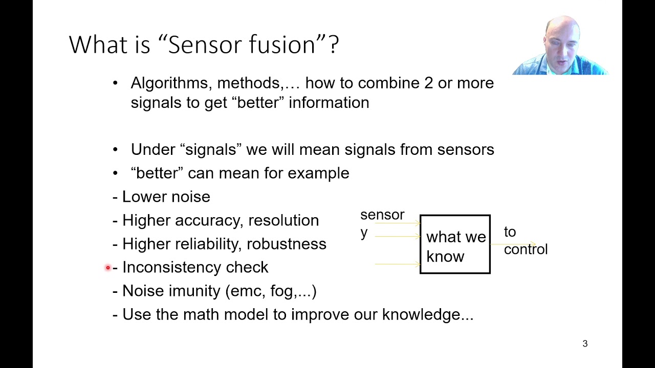





The Kalman Filter is an optimal recursive algorithm for estimating the state of a dynamic system from a series of noisy measurements. It operates in two iterative steps: prediction and correction. In the prediction step, the filter projects the current state estimate forward in time using the system's mathematical model, accounting for process noise. In the correction step, the filter incorporates the latest measurement to refine the prediction, using a weighted combination where the Kalman gain determines how much trust to place in the measurement versus the prediction. The Kalman gain is calculated based on the relative uncertainties of the prediction and measurement, ensuring optimal estimation performance. This approach is particularly useful when dealing with systems where direct observation is impossible or unreliable, such as tracking a ship's position in a harbor using indirect measurements.
Kalman Filter Explained: Equations & Ship Tracking Example
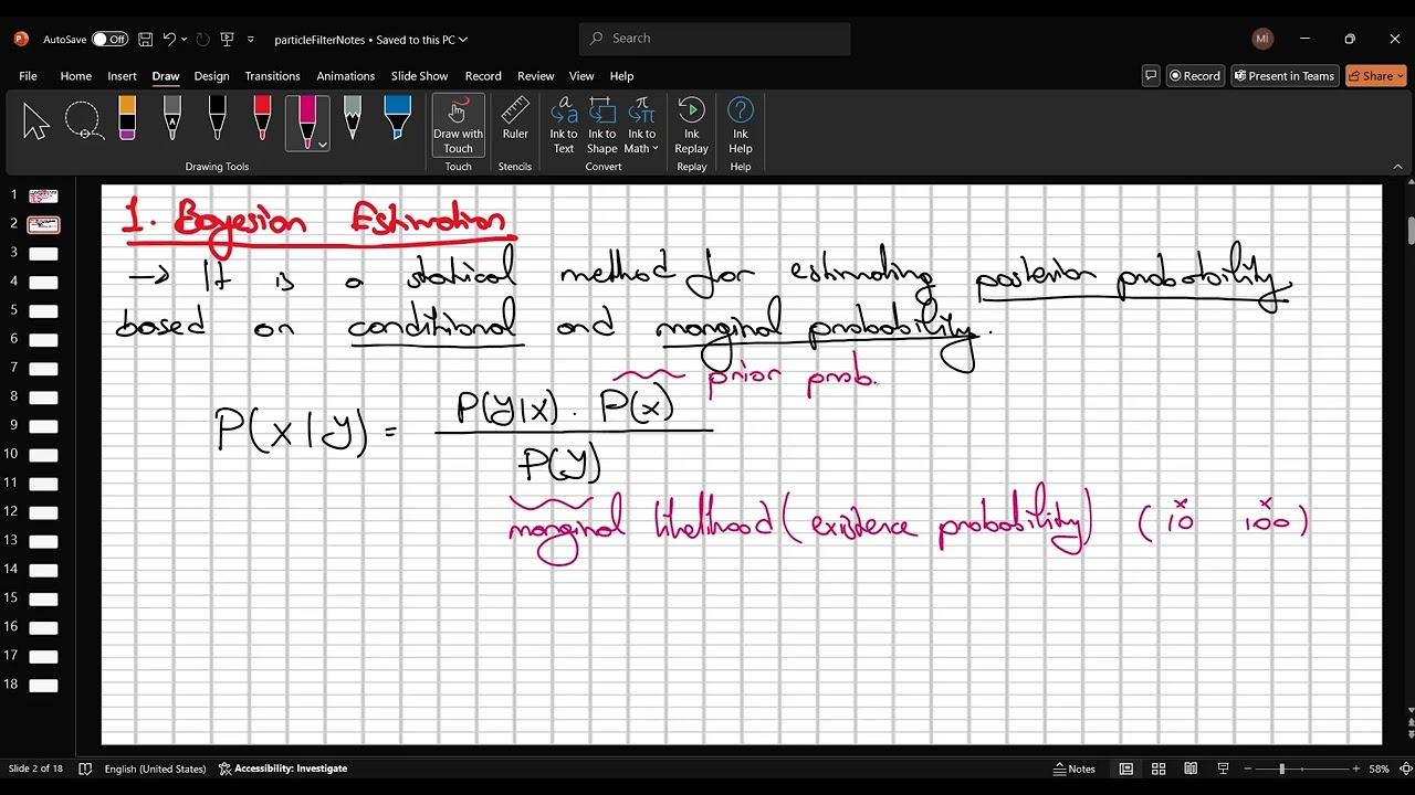
Added:what is the kalman filter well it's the optimal linear filter for discrete time systems so let's look at this set of equations here for a linear discrete time system we have the state vector x and i'll give an example in a minute but this is a vector here which represents the state of the system and this equation tells us how that state goes from time k to time k plus 1.
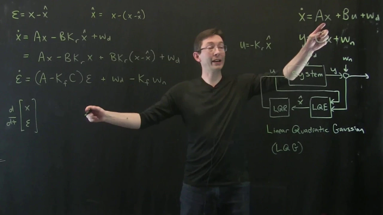
it's a linear set of equations so this state gets multiplied by a matrix the update matrix then there's also disruption that happens so there's noise that gets added to that and the noise here we're going to be assuming is gaussian but we could be more general that's multiplied by a matrix so this is a vector gaussian vector plus we're allowing for some deterministic inputs to this system and and that gets multiplied by a matrix again this is a vector so this is what we call our state space equation and then we're going to be observing that state through this equation here so we don't actually get to know what that state is and that's what the kalman filter is going to be doing it is going to be using these measurements to get estimates of the state so here's how you observe it you have the state multiplied by again it's linear multiplied by a matrix plus some gaussian noise of the observation which is in this case we're going to look at the case where it's independent of the noise that affected the system so let's look at an example when would this when would this uh be a practical system to you to consider well actually it's very very many cases but let's look at one here so let's think about a situation where we might have a ship in a harbor and we're trying to track the location of that ship as it moves in the harbor so we have east direction and north direction and we have an initial location for the ship and then we have some estimates of where that ship has moved so the ship will have moved and we are then going to be observing it not directly but through this equation and then we're going to see where we're going to ask ourselves questions like if it has moved from here to here where is it going to move next so can we predict using the kalman filter can we predict where it's going to go next and can we get a good estimate for where it is next after we make our next measurement or our next observation in this example here perhaps the the input the direct input would be the controls that the captain of the ship has applied to the ship these are deterministic that the captain's putting to maneuver the ship the w might be the waves and the wind which is disrupting the movement of the ship the x is the is a vector a two by one vector which is the amount of east and north uh in a vector that would be the state of the ship and then the observations might be for example a scaled version of the location like for example we might be looking at the ship let's say for example very simply simple examples we might be looking at the ship from above from a helicopter and the helicopter is looking through a a a a lens and that lens is scaling the location so they were getting a scaled version of the location at the x and y location the eastern north location plus there's some noise because the person who's looking through that lens is making some errors as they're estimating where that location is so that might be an intuitive example that matches these equations here so let's come back and think about this in a minute let's write down some of those strict uh assumptions we're making where the initial state of x is is unknown but has a mean of x tilde naught and a covariance of a matrix p naught we're just going to be assuming that in this system as i said w and v are zero mean gaussian and this equation here shows their the relationship between them so the expected value of this vector times itself transposed shows us that there's zeros on the off diagonal that's the one case we're going to consider here although there are more general versions so this tells us here that we're considering the case where there's no correlation between the noise in the state and the noise in the observations and this delta here tells us that these have the auto correlation only when k equals l so they're also independent in time so the w's and the v's are independent from one time to the next now here is our estimate this is what the kalman filter is going to be calculating for us so we're going to use a hat over the x to represent an estimate of x and what this notation means is that an estimate of x at time k given all of the observations up to k minus 1. so that's what this notation means and that is defined as being the expected value of x k the state vector the expected value of that given and we're going to use a capital z here is the collection of all the measurements up until time in this case k minus 1 so that's what the capital z means so this is a conditional probability where we're saying what is our expected value of x in this example down here what's our expected location given all the observations we've made up to time k minus 1 that's this equation here if we have x subscript k vertical line k that means the expected value of x given all of the measurements including the measurement at time k so that's the notation and here we have a matrix which is defined you can see here is a matrix which is the because this is a vector this is a row because there's a transpose and so this is the correlation matrix covariance matrix for the estimate so it's the expected value of the error this is the true location or the true state minus the estimated state and so this is a matrix which we're going to need in our filter as well so there's lots of equations and lots of notation i'm going to show you the equations now for the kalman filter and again there's lots of equations here but let's walk ourselves through them slowly so we really understand them so here is an update for our state estimate so this let's look at this one first what's happening in this equation i might just cover up the others so we're not distracted and let's look focus on this one here so this is saying that we are going to be first of all calculating what is the estimate of x at time k given the measurements up to k minus one that's what we defined over here and the kelvin filter says that we can work that out from the previous estimate at time k minus one given all the measurements up to time k minus one so if we've got that value then we can take that value which is the estimate at time k minus 1 which was based on all of the measurements up to time k minus 1. so everything we knew up to that previous time if we take that estimate multiply by f and we can see the matching that's going on here between the actual state and our estimate so our estimate is following the same form as our actual state so we're taking our estimate we're updating our estimate by multiplying by f which is getting to looking at the next time plus the deterministic input which we know about so we can take our previous estimate at time k minus 1 with all the measurements up to take time k minus 1 and we can work out this value over here that we defined so how should we think about this equation well this equation is an update equation because we're going from k minus 1 to k this is the update equation that we would make to our state estimate if we didn't actually have any new measurements okay so we've only got measurements up to k minus 1 but we'd like to predict where our new state is and so this is the equation that enables us to do that predicting into the future without having taken a measurement yet so then we can think to ourselves okay how do we update that once we do take a measurement at time k and that's what the next equation in the kalman set of equations is so here we have now the estimate at time k given that we've taken a measurement at time k and not surprisingly that equals the predicted state that we just worked out before we'd taken the measurement at time k so this was the best we could do at predicting what's happening at time k without having actually yet taken that measurement at time k that's this value here and then we're going to modify that in this case in the kalman filter case it's an addition of a term which depends on the measurement at time k okay so and this term depends on how much error there is between what we measure at time k and what we would have predicted to have measured so here if we if we again if we take our prediction without having yet taken the measurement if we take that and put it into this equation here we are going to where we multiply by h prime k we are going to get what we think we should be measuring okay and that's what this is here you can see it exactly it's x at time k given k minus 1 that's what we just calculated the best prediction we could have at time k before we actually take a measurement at time k multiply it by h prime k that will give us where we are expecting our measurement to be now a measurement is never exactly there because x hat is never exactly the state and also where there's noise in the measurement so there's an error term here and that error term gets multiplied by what we call a kalman gain okay so here's the two steps for updating our state space estimate and they're iterative because as each time k goes on you can put this one now into this with a different with the time offsets there goes into there you update the next one at the next time put this value into here and here you get the next one and you keep iterating these so this is the kalman filter giving you either one step ahead prediction or an estimate after you've made the measurement at time k so now the only thing we don't know is this kelman gain here so how do we calculate the kalman gain and so these are the other equations in the set of equations so here's the kalman gain it uses capital k because of kalman's name it's a bit confusing because there's a little k for the time but just to know that why we use the capital k there so we've got a capital k here at time k equals this covariance matrix over here times h and you can see all of the expressions here including this matrix here which is the noise correlation matrix from the measurements okay so let's now look at this how do we calculate this this terms here well we need to know this covariance matrix defined over here how do we calculate this well there's two equations for calculating this and again they are iterative equations uh where you first of all update uh to the next time what you are one step ahead without having taken a measurement and then you put that into here where you can then update to find this matrix after you have taken a measurement and again you iterate these two equations exactly as we iterated the state space estimation equations okay so let's finish by coming back to this example of the ship in the harbour just to really try to see a practical example of these two equations here so for example this as we said the ship has traveled around here so you might have the estimate here uh out at time one after measuring the the measurement at time one this might be the estimate at time two after measuring uh the z at time two uh this at 3 and so on and this one here at 4 let's say okay so what are these two equations let's really see this one so this equation here would take we're now trying to find out about time 5 okay so we want to know time five given the measurements up to time four so this is what we knew about at time four this is this one here so x of four four and we're trying to find x hat of five four okay so we find uh we can use this equation here to get a value uh which is a linear operation on this exact value here times this matrix f and let's say for example it put us here okay so this might be x hat of five given four this is where it this equation here tells us we think it's gone from here before we've taken the measurement at time five and then we need this equation here to take that value because this would be five four that value here to take that value and correct it after we've taken the measurement at time five so this would be z five that we'll be taking here so again this is an error term here so let's say for example we took an example where where h equals 1. let's just say this is the identity matrix just to make our life simple and let's say that this value over here let's say that that value there is z k okay so let's say this is z k here z k okay so this might be z five okay so let's say you've measured z five and this equation here predicted before you got a chance to measure that it predicted that the state space would be over here but now you've measured z5 over here so let's look at this term here this term is z5 minus this predicted value here and i said we're going to just simplicity consider h to be identity so that's this value here so this in the slide the square brackets here is the vector z k minus the this vector here so that is actually this vector here okay so inside the square brackets is that vector there and then you're going to multiply that vector by an amount given by the kelman gain and add it to this this location here so to get the overall update you're moving along here according to this equation you're moving along here by this amount that's this value here and then you are going to move along this direction according to what's in the square brackets by an amount given by the kalman gain and that is going to give you let's say for example that value took you to this point here so you've moved that far along uh the vector and that value there would be x hat of five given five okay so i just wanted to give this practical example and so you can sort of graphically see visualize what the what these equations are doing to an estimate of a state space in a in a two-dimensional example of tracking a ship in a harbor so hopefully this has given more insight into these equations if you found the video helpful give it a thumbs up it helps others to find the video check out the description below for more videos and there's a web page there where you'll find a full categorized listing of all the videos on the channel and of course subscribe to the channel for more videos you
Up Next

Creo Parametric: Chebyshev Lambda Linkage Mechanism Tutorial
@CADPLMGuy
9K views•2022-10-12

Ultrasonic Transducers: Resonant Frequency Measurement and Horn Design
@imajeenyus42
229.9K views•2017-02-22

Polymer Environmental Degradation: Mechanisms & Stabilization
@iit
1.8K views•2012-07-10

How a Student's Question Saved a NYC Skyscraper from Collapse
@veritasium
22.8M views•2025-04-26
Related Study Plans & Knowledge Roadmaps
Structured learning paths in Engineering